

You may remember covering the concept of convolution in Chapter_3, Module_4 of this course. Make sure you are acquainted with the one dimensional convolution therein. The mathematical treatment is easily extended from one dimension to two dimensions:

The symbol ** is used here to represent full convolution in two dimensions. Note that for each value of x and y the integral has to be evaluated over all values of x' and y'.
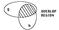
Such an operation can be thought of as an overlap intergral. The functions g and h are overlapped with a certain displacement between them and the total "weight" of the overlapping region is evaluated. The displacement is changed and the overlap re-evaluated. The process is repeated for all possible displacements.

For the discretely sampled datasets we are considering in this course such a summation would require a large number of computations (of the order M2N2). The Fourier transform of this convolution is given by F(u,v), where:

Alternatively this may be written using the Fourier operator F in a particularly simple and useful form:

The Fourier transform of a convolution is the product of the Fourier transforms of the functions.
Using the Fourier transform to evaluate a convolution requires of the order MNlog(M+N) operations, which is a considerable improvement over the simple summation method.


