|
|
 |
| Chap. 2 |
|
|
|
|
Chapter 2 Section B - Smoothing
Smoothing is often used to reduce the visible "noise" or random pixel
to pixel variations in images. It also provides a convenient
introduction to neighborhood operations.
Image noise is a random (or sometimes not so random) variation in pixel
values. Regions that should be perfectly uniform have peaks in the
histogram whose width is a measure of the amount of variation. Some of
this comes from the statistical variation in the finite number of
photons or electrons that are collected in the camera to represent each
pixel. This is primarily an important factor when dealing with X-ray
images from the SEM, radiographic images, electron images, or
fluorescence images. The number of photons in even a short exposure
picture captured in the light microscope or with a macro camera is
usually very large so that the statistical variation is quite small.
There are exceptions of course, such as astronomy and flourescence
microscopy.
Noise can also be introduced by electronic effects in the camera,
amplifier, or digitizer. Some of these contributions (such as the
thermal noise that causes variations in the signal as it is passed from
one transistor to another within a solid state camera) are also random
(although for common CCD cameras they typically vary im amplitude from
one side of the image to the other, and with brightness), but many of
them are not and show up as periodic fluctuations. For example, the
vertical lines that appear in the several of the images (particularly
after processing such as local equalization, discussed in Chapter 3)
are due to noise in the digitizer which caused even and odd addresses
along each scan line to vary slightly. The pattern is invisible in the
original image but becomes "enhanced" by processing. Many of these
systematic sources of noise can be removed in the Fourier or frequency
domain representation of the image more easily than in the spatial
domain (pixel) images, as discussed in Chapter 4.
|
|
|
 |
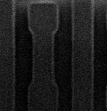
| This
example, shows an SEM image of an integrated circuit (Singlefra). Using
only a single video rate raster scan and a low accelerating voltage (to
minimize specimen charging and damage) produces a small number of
electrons and hence a noisy image. |
|
|
|
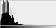
The histogram shows the amount of scatter in the values. In addition to
the scatter, there is a pronounced even-odd effect in which the analog
to digital converter used to digitize the image has biased the process
so that pixels are more likely to be assigned an odd brightness value
than an even one.
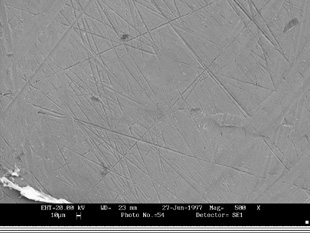
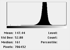
Noise due to counting statistics is most directly reduced by signal
averaging over time (temporal averaging). Some video cameras and some
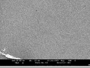
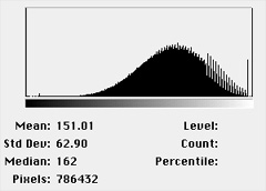
frame grabbers allow integration over a period of time. In the example
shown below the scan rate of the SEM is varied to collect two images
from the same area, one in a few seconds and one in 100 seconds. The
histograms show the marked reduction in variation across the uniform
sample area when more signal is collected. Reducing the noise allows
the surface scratches to be seen.
|
|
|
 |
| SEM_Fast image and histogram. |
|
|
|
|
 |
| SEM_Slow image and histogram. |
|
|
|
Smoothing (practically all programs have some built-in "smoothing"
operator that averages each pixel with its neighbors) is usually done
by simply adding the values together and dividing by the number of
pixels, or by using a predefined set of weights that increase the
contribution of the central pixel. The simplest Photoshop smoothing
function is called Blur. Select Filter -> Blur -> Blur,
or Blur More. There is no specific documentation on the particular
weight values used in these functions; the Blur function appears to use
a kernel (as defined below) with weights (0 1 0) (1 4 1) (0 1 0). It is
extremely fast to apply.
User-defined kernels or sets of weights can also be used. These will be
employed in later operations for other image processing purposes, such
as edge enhancement. They are generally described as kernel or
neighborhood operations, or as linear operators. With an appropriate
set of weights, operations described variously as smoothing,
differentiation, gradient and edge operators, low-pass or high-pass
filters, etc., can be performed. Photoshop provides several ways to
apply such kernels. Select Filter -> Other -> Custom
and either enter various kernel values or load predefined sets from
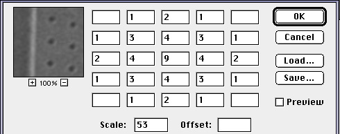
disk. These can be up to 5 x 5 pixels in size. For example, you could
enter a set of weights by hand into the dialog box as shown below.
|
|
|
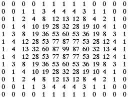
Notice that the weights consist of small integers arranged
symmetrically around the center, dropping in magnitude in a
more-or-less Gaussian relationship with distance. This is a classic
smoothing kernel. Such a set of weights is typically described by the
standard deviation of the Gaussian curve which they approximate. Notice
also that the sum of the weight values has been entered manually into
the "Scale" field. This is used to divide the sum of the products of
the pixel values times the weights, so that the resulting value lies
within the 0..255 range of brightness values for grey scale pixels. The
Offset field is not used with sets of weights that are all positive;
future examples with negative values will show an entry there as well.
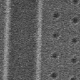
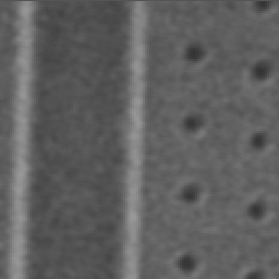
When the image has noise present in the most common form - a random
variation of the individual pixels due to a low signal strength -
averaging with a center-weighted kernel of values can reduce the
visible effects of the noise. The specific values can either be
calculated from a Gaussian or simply entered by hand empirically, being
sure that you keep them symmetrical about the center and enter the
total of the positive values as the scale.
|
 |
| Original image. |
|
 |
| Smoothed result. |
|
|
|
There are typically several sets of weights provided with Photoshop
that include some smoothing operators, or you may experiment with your
own or enter values from references such as The Image Processing
Handbook. The live Preview window in the dialog gives useful feedback
on the results of changes in the weights.
The built-in "Custom" filter in Photoshop allows you to interactively
enter coefficients into the kernel while seeing a preview of the effect
on the image, and is a very good way to learn about convolution
kernels. It has several limitations, however: 1) only integer values
can be used; 2) it only works with 8 bit per channel images, not 16 bit
images; 3) there is no way to automatically scale the result to the
dynamic range of the image; and 4) it is restricted to a small 5x5
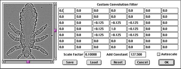
neighborhood. The Filter -> IP*Process -> Custom
filter overcomes these limitations. You can enter up to a 7x7 array of
floating point values, as well as loading kernel files on disk (in both
the Photoshop *.acf format and the text file format used by the Filter -> IP*Process -> Convolution
function - in the latter case the 7x7 central portion of larger kernels
is used). The filter can be applied to both 8 and 16 bit per channel
grey scale and RGB color images, there is a check box to force the
results to be autoscaled to fit the dynamic range of the image, and
there is a large preview window to show the results interactively.
Filter values are recorded in Photoshop Actions and can be saved on
disk (in text file format). Filter values can range from 0.0001 to
10000, and all of the math is performed internally with double
precision floating point arithmetic to preserve the accuracy of results
when kernels or images contain both large and small values.
|
|
|
For even larger kernels (up to 95x95), arrays of values in either
integer or floating point format can be created as text files (*.txt)
for use by the Filter -> IP*Process -> Convolve
plug-in. Files must consist of an array of values, separated by tab,
comma or space, and arranged in an array that is square and odd in
dimension (3x3, 5x5, 7x7, ... 95x95). These can be entered using
SimpleText on the Mac or NotePad under Windows, or using a spreadsheet
program and saving the file in plain text format. Several examples are
provided on the CD-ROM in a folder named Kernels. The plug-in reads the
file values and allows the user to choose several modes of automatic
scaling of the results, and applies it to the image. The name of the
kernel file is recorded in Actions so that different convolution
kernels can be applied automatically.
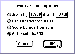
There are several options for scaling the result of the convolution.
The most common is to divide the sum of the products of the pixel
values and weights by the sum of the positive values in the kernel; in
the smoothing example, where all of the values are positive, this is
simply the sum of all the values. For the cases shown below in which
negative values are used, it is common to use an offset value of 128
(medium grey) so that results in which the sum of the products may be
negative are not simply clipped to black, and the dark details can be
seen. The plug-in also allows the user to enter other scaling and
offset values, or to select auto-scaling in which the values are
automatically adjusted to produce a full grey scale dynamic range.
|
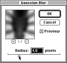 There is also a built-in Gaussian filter. Select Filter -> Blur -> Gaussian Blur or Filter -> IP*Process -> Gaussian Blur
and specify the radial standard deviation of the Gaussian function by
using the slider. Increasing the standard deviation increases the
amount of the blur as shown in the live Preview window.
|
|
Conditional smoothing (Filter -> IP*Process -> Cond.Smooth)
attempts to use weighted averaging of pixels in a neighborhood while
reducing the blurring of images. Weights for each pixel are calculated
according to the distance of the pixel from the center of the
neighborhood and the difference between the pixel value and the central
pixel. Pixels that are very different from the center pixel are
weighted less, because they may lie on the other side of a boundary. As
shown in the example (an enlarged portion of the Lena image with added
noise), edge detail does remain sharp while pixel-to-pixel noise
variation is reduced. However, superior results are usually achieved
with a median filter as discussed in the next section.
|
|
Enlarged fragment of the original Lena image with added noise.
|
|
Result of conditional smoothing.
|
|
Result of median filtering.
|
|


 There is also a built-in Gaussian filter. Select Filter -> Blur -> Gaussian Blur or Filter -> IP*Process -> Gaussian Blur
and specify the radial standard deviation of the Gaussian function by
using the slider. Increasing the standard deviation increases the
amount of the blur as shown in the live Preview window.


