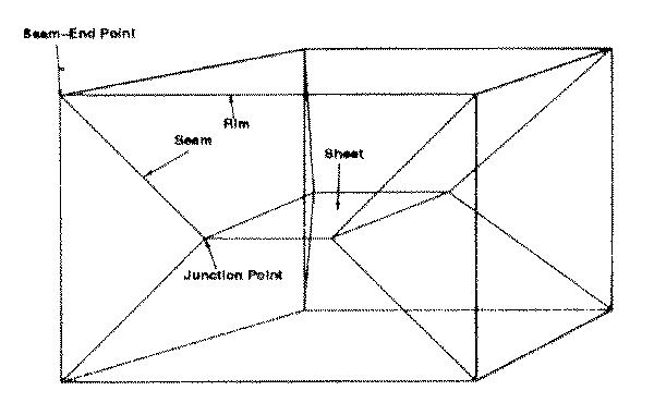
Fig.1 : Sheets, Seams and Rims (from [Sherbrooke96]).
Providence, April 27, 1998
Presented by Frederic Leymarie
Brown University
ToC:
Mathematical Morphology : 3D Thinning
Computational Geometry: Polyhedra & Max. Inscribed Spheres
Wave Propagation: Cellular automata & Distance Transforms
Initial assumptions:
In other words: "We have a bounded section of an equidistantly sampled Euclidean space of dimension D=3."
This is also called:
Early work by Lobreght in 1980 who used the Euler number to determine when to remove a voxel :
Sufficiency condition:
Toriwaki showed (1982) that a an additional condition was required: only one "cluster" of voxels (a single and simply connected set) should be attached to the central voxel, to be removed.
Near Euclidean metric
Verwer (1991) introduces "bucket sorting" to minimize voxels' status update. This is done by ordering voxels in terms of distance to the object's surface. It optimizes numerical complexity and permits to use near Euclidean metrics (integer or vector-based).
Jonker (1995) answers the following questions:
Specificity of Thinning:
"Thinning algorithms operate within an image on the objects, to which connectivity can be associated."
Definition of skeletonization in 3D - notion of Dimensional Reduction :
Connectivity paradox (of squared/cubical grids):
An object (foreground or FG) can pass through the background (BG) when it shouldn't and vice-versa (in 2D this leads to the 4-connected - 8-connected distinction between FG and BG). In 3D, we get the following choices to resolve the "paradox":
Euclidean metric:
Firstly, perform an EDT (Euclidean Distance Transform) to assign a distance value to each object voxel. The EDT is a mapping from a two-valued set (object - background) to a multi-valued set, where distance values (from the object's boundary) are assigned to the background (or to the interior of the object).
Secondly, do the thinning in order of increasing distance.
In 2D, this is equivalent to representing the object by sets of (convex) polygons and deriving an analytic locus of symmetries (e.g. cf. Preparata in 1977). Thus, most of the perspiration is spent on obtaining a valid representation of an object in terms of polygons (in 2D) or polyhedra (in 3D).
This approach is strongly influenced by CSG (Computational Solid Geometry) representations in use within CAD-systems. In other words, the usefulness of the method is driven by applications to "human-made" objects, as modeled today in computer systems. Many references in the recent literature, through the 80's and 90's.
Fig.1 : Sheets, Seams and Rims (from [Sherbrooke96]).
N.B.: Connected components of end points are called rims (our "ribs").
The properties of the Delaunay triangulation of point sets has been exploited as a means of skeletal construction in both 2D and 3D. E.g. Yu et al. (1991) relies on the 3D Delaunay triangulation of a dense distribution of points lying on the boundary of the solid. It is demonstrated that the circumspheres of the resulting tetrahedra approximate maximal spheres.
Given a set S of N distinct points p1, p2, ... pN, in R3, each point pi in S can be associated with a unique polyhedron vi, 1 <= i <= N, where vi is the locus of all points x in R3 that are closer to pi than to any other point of S i.e.,
vi = { x : d(x , pi) < d(x , pj) , for all i not j , pi, pj in S }
where d is the Euclidean distance. vi is an open convex polyhedron sometimes referred to as the Voronoi polyhedron or Voronoi region.
The Delaunay triangulation of S consists of the set of tetrahedra formed by connecting the neighboring points pi and pj between the adjacent polyhedra vi, vj.
A fundamental property of the Delaunay triangulation of S is the empty circumsphere property. The circumsphere associated with each Delaunay tetrahedron does not contain any points of S in its interior. This is a direct consequence of the Voronoi construction since the vertices of the Voronoi diagram are the circumcenters of the associated tetrahedra.

Fig.2 In 2D, the circumcircle of a Delaunay triangle
approximates an inscribed circle (from [Sheehy96]).
Given a set of points S lying on the boundary of a solid T and its corresponding Delaunay triangulation, it can be demonstrated that as S becomes infinitely dense the circumsphere associated with each tetrahedron in the interior of T tends to a maximal sphere and its circumcenter to a point on the medial surface.
Generating and triangulating an infinitely dense distribution of points is not possible in practice. From sparse sets however, the approach is practical and leads to the correct topology.
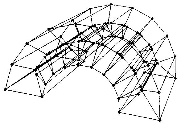
Fig.3 Boundary & MA of a 30-element shell (from [Sherbrooke96]).
In an attempt to address problems of previous approaches as well as going further ahead in designing a powerful process for shape description and representation we propose a "new" approach for dealing with symmetry elicitation in 3D.
What we are aiming at:
Let Phi(q0,t) be the wavefront of the point q0 after time t. For every point q of this front, consider the wavefront after time s: Phi(q,s).
Then, the wavefront of the point q0 after time s+t, Phi(q0, s+t), will be the envelope of the fronts Phi(q,s), such that q in Phi(q0,t).

Fig.4 Illustration of Huygens'
principle.
In this formulation, one can replace the "point" q0 by a curve, surface, or in general, by a closed set.
Furthermore, the 3D space can be replaced by any smooth manifold, and the propagation of light can be replaced by the propagation of any disturbance transmitting itself "locally" [Arnold89].
We can also replace the metric from Euclidean to a Riemannian, and model anisotropic "shape" properties (of the medium, or space).
The difficulty, is to translate this principle in a discrete world relying upon a lattice, such as the X-Y-Z grid made of voxels, traditionally used in image processing.
We have developed such a "discrete" method relying upon a 3D grid. We call it 3D-CADT for:
In this approach, we simulate propagation of information by the use of a class of cellular automata "oriented" in the direction of the wavefront. Equivalently, these automata rely upon the metric characteristic of the underlying space (the "indicatrix"). For Euclidean 3D space, this is a sphere or directions.
The resultant ray system, is the system of normals to a surface in Euclidean space. In the ngb. of a smooth surface, its normals form a smooth fibration, until at some distance from the surface, various normals may begin to intersect one another.
Historical note: These "singularities" were first investigated by Archimedes (caustics of light rays, around 300 B.C.).
Fig.5 Initial level sets (d=3) from a sphere and a plane
together with
resultant medial axis (a parabola).
Fig.6 Initial level sets (d=10) from a sphere and a
plane together with
resultant medial axis (a parabola).
Fig.7 Initial level sets (d=5) from a cylinder together
with
resultant medial axis (a "stick").

Fig.8 "Peter's" object : z1 = (ay+b)x^2
(b>0) , z2 = cx + dy + e (e > 1/2b)
Fig.9 The computed skeleton for Peter's object.
3D shocks have been proposed by Kimia.These are based on curvature properties of a level hypersurface, £, in a 4D space which represents the evolution of a 3D object under a wave propagation (or under a motion defined by a so-called "reaction-diffusion" PDE).
Shock type |
Gradient |
Principal curvatures |
1-n |
£' disc. |
Undefined |
2-1 |
£' = 0 |
K1.K2 < 0 & K3 != 0 |
2-2 |
£' = 0 |
K1.K2 < 0 & K3 = 0 |
3-1 |
£' = 0 |
K1.K2 > 0 & K3 = 0 |
3-2 |
£' = 0 |
K1=K2=0 & K3!=0 |
4 |
£' = 0 |
K1.K2 > 0 & K2.K3 > 0 |
Figure 10: The 4 classes of shocks
Page created by Frederic
Leymarie, 1998.
Comments, suggestions, etc., mail to: leymarie@lems.brown.edu