
Brush Rasterization
\(\newcommand{\bm} [1]{ \mathbf{#1}}\) \(\newcommand{\reals}{ {\rm I\!R}}\) \(\newcommand{\trsp}{ {{\scriptscriptstyle\top}}}\)
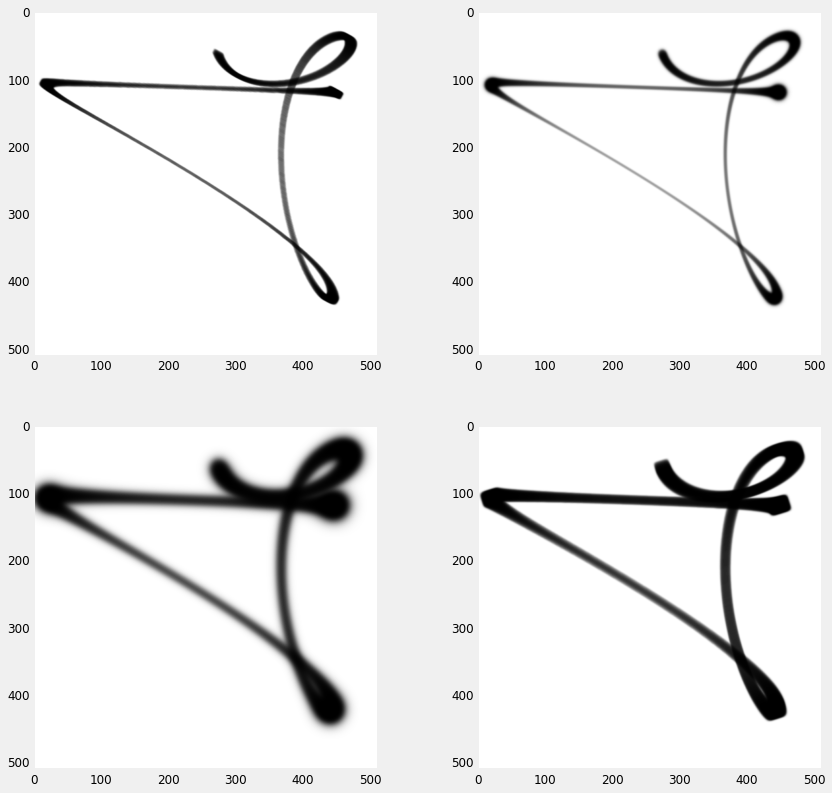
One of the advantages of generating curves through the simulation of a movement, is that the smooth kinematics can be exploited to implement more expressive rendering methods. Here we demonstrate a simple brush model, that assumes that the amount of paint deposited is inversely proportional to the speed of the pen. While this is obviously not an accurate model of a brush or pen, it results in renderings that do accentuate the perceived dynamism of the trace.
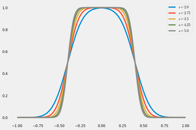
To render a brush we want a variably smooth texture, one possible way of doing
so is to create a hat function. This can be done with an "S" shaped function,
such as the s-curve
\[
f(t) = -1 + \frac{2}{(1 + e^t)},
\]
the error function (\(\mathrm{erf}\)) or the hyperbolic
tangent (\(\mathrm{tanh}\)).
import cv2
import matplotlib.pyplot as plt
import matplotlib.image as mpimg

from scipy.special import erf

def scurve(t):
    return 1. / (1. + np.exp(-t))*2. - 1.

def hat(x, sharpness, func=erf):
    # Can use tanh instead...
    return (func((1.-np.abs(x*2.5))*sharpness)*0.5+0.5)

x = np.linspace(-1,1,200)
plt.figure(figsize=(10,7))
for s in np.linspace(2., 5, 5):
    plt.plot(x, hat(x, s), label='$s='+str(s)+'$')
plt.legend()
plt.show()
To generate an image compactly we can take advantage of a nice NumPy trick, where adding a row and a column vector produces a matrix:
x = np.linspace(1, 5, 5) # row
y = np.linspace(1, 5, 5).reshape(-1, 1)
m = x + y
# SimPy (used for latex rendering) considers numpy arrays with one dimension as column vectors,
# so we explicitly set it as a row here
latex(x.reshape(1,-1),'x'), latex(y,'y'), latex(m,'x+y')
| \[x=\left[\begin{matrix}1.0 & 2.0 & 3.0 & 4.0 & 5.0\end{matrix}\right]\] | \[y=\left[\begin{matrix}1.0\\2.0\\3.0\\4.0\\5.0\end{matrix}\right]\] | \[x+y=\left[\begin{matrix}2.0 & 3.0 & 4.0 & 5.0 & 6.0\\3.0 & 4.0 & 5.0 & 6.0 & 7.0\\4.0 & 5.0 & 6.0 & 7.0 & 8.0\\5.0 & 6.0 & 7.0 & 8.0 & 9.0\\6.0 & 7.0 & 8.0 & 9.0 & 10.0\end{matrix}\right]\] |
We can then apply then use the "hat" function to generate a variably smooth brush texture.
import scipy.ndimage as ndimage
def hat_img(radius, smoothness, center=np.array([0,0]), func=erf):
    size = int(radius)*4 # image size
    center = np.array(center)/radius # center (for subpixel rendering)
    x = np.linspace((-size/2)/radius - center[0], (size/2)/radius - center[0], size+1)
    y = np.linspace((-size/2)/radius - center[1] , (size/2)/radius - center[1], size+1).reshape(-1,1)
    img = (x**2 + y**2)
    img = hat(img, smoothness, func) #scurve)
    return img
img = hat_img(64, 10, center=[0.0,0.])

plt.figure(figsize=(8,4))
plt.subplot(1,2,1)
img = hat_img(64, 10, center=[0.0,0.])
plt.imshow(img*255, interpolation='bilinear')
plt.subplot(1,2,2)
img = hat_img(64, 1, center=[0.0,0.])
plt.imshow(img*255, interpolation='bilinear')
plt.show()
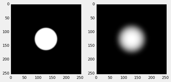
Note that it is important to use bilinear intepolation in imshow, othewise Matplotlib will
create artifacts when rendering (which made me loose tons of time!).
The center parameter in the hat_img function will allow us to render the brush at
sub-pixel positions, which would be trivial in OpenGL but needs to be taken care
of here to avoid rendering artefacts.
A more interesting and flexible brush texture can be generated with a super-ellipse
#length(max(abs(p)-b,0.0))-r;
def hat_img(w, h, theta, power, smoothness, center=np.array([0,0]), func=erf):
    radius = max(w, h)
    size = int(radius)*4 # image size
    print w/radius, h/radius
    center = np.array(center)/radius # center (for subpixel rendering)
    x = np.linspace((-size/2)/radius, (size/2)/radius, size+1)
    y = np.linspace((-size/2)/radius, (size/2)/radius, size+1).reshape(-1,1)
    # rotation
    ct, st = np.cos(theta), np.sin(theta)
    xr = x * ct - y * st - center[0]
    yr = x * st + y * ct - center[1]
    ratio = 0.5
    # scale
    x = xr / (float(w)/radius)
    y = yr / ((float(h)/radius))
    # superellipse distance
    img = np.sqrt(abs(x**power) + abs(y**power))
    img = hat(img, smoothness, func)
    return img

plt.figure(figsize=(8,4))
plt.subplot(1,2,1)
img = hat_img(64, 24, 0.6, 4.0, 10, center=[0.0,0.0])
plt.imshow(img*255, interpolation='bilinear')
plt.subplot(1,2,2)
img = hat_img(64, 24, -0.3, 8.0, 2, center=[0.0,0.0])
plt.imshow(img*255, interpolation='bilinear')
plt.show()
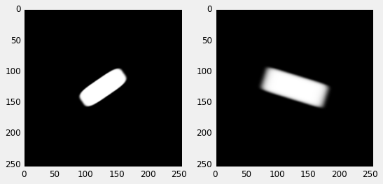
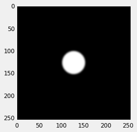
which still allows us to generate a round brush (with a power of \(2\))
img = hat_img(64, 64, 0.0, 2.0, 10, center=[0.0,0.0])

plt.imshow(img*255, interpolation='bilinear')
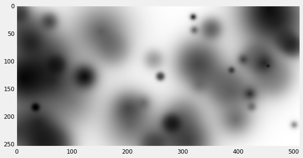
We can now apply the texture to a second image with alpha blending in order to generate patterns
img = np.zeros((256,512))

alpha_blend = lambda a, b, alpha: a*(1-b*alpha) + b*alpha

def draw_brush(img, pos, w, h, theta, power, smoothness, func=erf, alpha=1.):
    px, py = np.array(pos)
    im_h, im_w = img.shape

    round = lambda v : int(np.floor(v))

    # subpixel position
    center = np.array([px-round(px), py-round(py)])

    pimg = hat_img(w, h, theta, power, smoothness, center=center, func=func)
    ph, pw = pimg.shape

    # texture position
    x1 = round(px) - pw/2
    y1 = round(py) - ph/2
    x2 = x1 + pw
    y2 = y1 + ph

    # culling
    if x1 < -pw or y1 < -ph:
        return
    if x1 >= im_w or y1 >= im_h:
        return

    # clip
    ox1 = abs(min(x1, 0))
    oy1 = abs(min(y1, 0))
    ox2 = max(x2 - im_w, 0)
    oy2 = max(y2 - im_h, 0)

    # blit
    img[y1+oy1:y2-oy2, x1+ox1:x2-ox2] = \
    alpha_blend( img[y1+oy1:y2-oy2, x1+ox1:x2-ox2], pimg[oy1:ph-oy2, ox1:pw-ox2], alpha)

def draw_radial_brush(img, pos, radius, smoothness, func=erf, alpha=1.):
    draw_brush(img, pos, radius, radius, 0., 2., smoothness, func, alpha)

# Draw some random particles
np.random.seed(23)
# random point on matrix
rand_2d = lambda shape: [np.random.uniform(0, shape[1]),
                         np.random.uniform(0, shape[0])]

for i in range(50):
    draw_radial_brush(img,
                  rand_2d(img.shape),
                  np.random.uniform(5,100),
                  np.random.uniform(1.0, 4.),
                  func=scurve,
    alpha=np.random.uniform(0.3,1.))

img = 1. - img

plt.figure(figsize=(10,5))
plt.imshow(img, interpolation='bilinear')
plt.show()
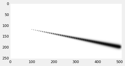
or to render a variable width line, in a process commonly known as "dabbing" or "stamping"
img = np.zeros((256,512))

n = 50
pts = np.vstack([np.linspace(100, 500,n), np.linspace(120,200,n)])
R = np.linspace(2, 16, n)
for p, r in zip(pts.T, R):
    draw_radial_brush(img,
                  p,
                  r,
                  1.1,
    func=np.tanh)

img = 1. - img

plt.imshow(img, interpolation='bilinear')
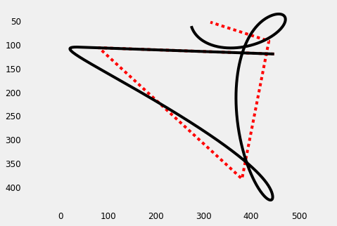
The same method can be used to generate "brushy" renderings of a movement path. Here we test it with a spring-damper system that follows a target along a linear path.
from scipy.interpolate import interp1d
def spring_path( P, duration, kp, damp_ratio, dt ):
    kv = damp_ratio * 2. * np.sqrt(kp)
    m = P.shape[1]
    n = int(duration / dt)
    # equilibrium point
    ft = interp1d( np.linspace(1, m, m), P, 'linear' )
    x_hat = ft(np.linspace(1, m, n))
    # output
    y = np.zeros((2, n))
    # current pos and velocity
    x = x_hat[:,0]
    v = np.zeros(2)
    # Euler integration
    for i in range(n):
        y[:,i] = x
        f = - v*kv + (x_hat[:,i] - x)*kp
        v += f*dt
        x += v*dt
    return y

np.random.seed(10)
P = np.random.uniform(10, 500, size=(2,5)) + np.array([60,0]).reshape(-1,1)
X = spring_path(P, 2., 100., 0.1, 0.001)
plt.figure(figsize=(7,5))
plt.plot(P[0,:], P[1,:], 'r:')
plt.plot(X[0,:], X[1,:], 'k')
plt.axis('equal')
plt.gca().invert_yaxis()
plt.show()
To add a sense of dynamism to the image, we vary the size of the brush with an inverse function of the istantaneous speed \[ w_t = w_{min} + (w_{max} - w_{min}) \mathrm{exp} \left( { -\frac{ \left| \dot{x}_t \right| }{\mu_x} } \right) \]
def brush_w(X, minw, maxw):
    # compute speed, no need for dt since we normalize
    dX = np.gradient(X, axis=1)
    s = np.sqrt(np.sum(dX**2, axis=0))
    w = np.exp(-s / (np.mean(s)+1e-100))
    return minw + (maxw-minw)*w

img = np.zeros((512,512))

def brush_path(img, X, minw, maxw, ratio, theta, power, smooth=2.3):
    W = brush_w(X, minw, maxw)
    for p, w in zip(X.T, W):
        draw_brush(img,
                  p,
                  w,
                  w*ratio,
                  theta,
                  power,
                  smooth,
                  alpha=0.2,
        func=np.tanh)


plt.figure(figsize=(13,13))
plt.subplot(2,2,1)
img = np.zeros((512,512))
brush_path(img, X, 5, 15, 0.5, -0.5, 5.)
img = 1. - img
plt.imshow(img, interpolation='bilinear')

plt.subplot(2,2,2)
img = np.zeros((512,512))
brush_path(img, X, 3, 20, 1., 0.0, 2.)
img = 1. - img
plt.imshow(img, interpolation='bilinear')

plt.subplot(2,2,3)
img = np.zeros((512,512))
brush_path(img, X, 10, 25, 1.0, 0.0, 2., 1.)
img = 1. - img
plt.imshow(img, interpolation='bilinear')

plt.subplot(2,2,4)
img = np.zeros((512,512))
brush_path(img, X, 8, 20, 0.8, 0.3, 5.)
img = 1. - img
plt.imshow(img, interpolation='bilinear')

plt.show()
Created: 2017-04-17 Mon 14:56