
Generating Calligraphic Trajectories with Model Predictive Control (MPC)
Table of Contents
\(\newcommand{\bm} [1]{ \mathbf{#1}}\) \(\newcommand{\reals}{ {\rm I\!R}}\) \(\newcommand{\trsp}{ {{\scriptscriptstyle\top}}}\)
This document provides the Python source code for most parts of the methods described in the following papers:
Generating Calligraphic Trajectories with Model Predictive Control
@inproceedings{BerioGI2017,
 author = {Berio, D and Calinon, S. and Fol Leymarie, F.},
 title = {Generating Calligraphic Trajectories with Model Predictive Control},
 booktitle = {Proceedings of Graphics Interface},
 series = {GI 2017},
 year = {2017},
 address = {Edmonton, Canada},
 month = {May},
 publisher = {Canadian Human-Computer Communications Society},
}
and
Dynamic Graffiti Stylisation with Stochastic Optimal Control
@inproceedings{BerioMPCMOCO2017,
 author = {Berio, D and Calinon, S. and Fol Leymarie, F.},
 title = {Dynamic Graffiti Stylisation with Stochastic Optimal Control},
 booktitle = {ACM Proceedings of the 4th International Conference on Movement and Computing},
 series = {MOCO '17},
 year = {2017},
 month = {June},
 address = {London, UK},
 publisher = {ACM},
 address = {New York, NY, USA},
}
If some parts of the code were useful for your research of for a better understanding of the algorithms, please reward the authors by citing the related publications.
The source code for the whole document and necessary data files are available at this address:
1 Overview
Many computer aided design applications require the definition of continuous traces, where the most common interface is to edit the control points of some form of interpolating spline. We study how tools from computational motor control can be used to extend such methods to encapsulate movement dynamics, variations and coordination. Here we describe a methodology for the interactive and procedural definition of motion trajectories using stochastic optimal control.
Our system is based on a probabilistic formulation of Model Predictive Control (MPC) [Calinon2016] and provides users with a simple interactive interface to generate multiple movements and traces at once, by visually defining a distribution of trajectories rather than a singleunnpath. By exploiting this representation, a dynamical system is then used to generate curves stochastically.
The input to our method is a sequence of states defined as multivariate Gaussians with full covariances, which allow the manipulation of the curvilinear evolution as well as the variability of trajectory segments. The output is a trajectory that is consistent with the minimal intervention principle [Todorov2004], and minimises a tradeoff between control effort and tracking accuracy.
Full covariances allow the user to define coordinations and directional trends in the trajectory evolution, where an increase in variance produces a smoothing effect, which can be interpreted as a form co-articulation [Flash2005].
Gaussians with isotropic covariance can be used for emulating Bézier curves [Egerstedt2004], as well as for generating paths that minimise high-order derivatives of position, such as jerk [flash1985coordination], snap [Edelman1987] or crackle [Dingwell2004].
We propose our method as a general-purpose tool for motion synthesis and robotics applications. In addition, we support the hypothesis that the observation of a human made artistic trace triggers the mental recovery of the movement underlying its production [freedberg2007motion,pignocchi2010], and that this recovery affects aesthetic appraisal [DePreester2014]. As a result, we emphasise the advantages of the proposed methodology for the computational synthesis of hand drawn curves.
The following document describes the implementation of our system using Python. The code depends on the NumPy, SciPy and Matplolib libraries for the main functionality and on SymPy and svgpathtools packages for additional functionality. Note that some function and variable definitions that are not indenspensable for describing the method (and rather used for figures, loading data and formatiing the document) are hidden. The full source code and data files can be downloaded here:
2 Implementation
2.1 Dynamical system
We model the movement of a pen trajectory by optimising the evolution of a \(n\mathrm{th}\) discrete linear time invariant (dLTI) system with the state space representation \[\bm{x}_{t+1} = \bm{A}\bm{x}_t + \bm{B}\bm{u}_t,\] where the state is given by the position concatenated with its derivatives up to the order \(n-1\). The dynamics of the system are determined by the matrices \(\bm{A}\) and \(\bm{B}\), which fully describe the response of the system to an input command \(\bm{u}_t\). The output of the system is then given by \[ \bm{y}_t = \bm{C}\bm{x}_t \] where \(\bm{C}\) is the sensor matrix, which determines which elements of the states are taken into consideration (observed). We can implement the dynamical system as follows
#%%

import numpy as np

class DynSys:
    def __init__(self, order, dt=0.01, dim=2):
        self.order = order
        self.dim = dim
        self.dt = dt

        ## construct system matrices
        # continuous single
        A = np.zeros((order,order))
        A[0:order-1, 1:order] = np.eye(order-1)
        B = np.zeros((order,1))
        B[-1,:] = 1.

        # Euler discretization
        A = np.eye(A.shape[0]) + A * dt
        B = B * dt

        # Multiple output
        # Add dimensions
        A = np.kron(A, np.eye(dim))
        B = np.kron(B, np.eye(dim) )

        # Sensor matrix (assuming only position is observed)
        # Actually unused here and directly setting unobserved Q entries to 0 weight
        C = np.kron( np.hstack([np.ones((1,1)), np.zeros((1, order-1))]),
                    np.eye(dim))

        self.A, self.B, self.C = A, B, C

    def y(self, x):
        ''' y = Cx'''
        return np.dot(self.C, x)

    def num_timesteps(self, duration):
        return int(duration/self.dt)

    def matrices(self):
        return self.A, self.B

sys = DynSys(2)
latex(sys.A,'\\bm{A}'), latex(sys.B, '\\bm{B}'), latex(sys.C,'\\bm{C}') # show latex
| \[\bm{A}=\left[\begin{matrix}1.0 & 0.0 & 0.01 & 0.0\\0.0 & 1.0 & 0.0 & 0.01\\0.0 & 0.0 & 1.0 & 0.0\\0.0 & 0.0 & 0.0 & 1.0\end{matrix}\right]\] | \[\bm{B}=\left[\begin{matrix}0.0 & 0.0\\0.0 & 0.0\\0.01 & 0.0\\0.0 & 0.01\end{matrix}\right]\] | \[\bm{C}=\left[\begin{matrix}1.0 & 0.0 & 0.0 & 0.0\\0.0 & 1.0 & 0.0 & 0.0\end{matrix}\right]\] |
Note that here we formulate the sensor matrix \(\bm{C}\) in order to observe position only, since we are interested in specifying the evolution of the system with position constraints only.
2.2 Quadratic Cost Function
An optimal trajectory is computed by minimising a quadratic cost function that, for each time step, tries to reduce deviations from a reference state sequence while keeping the amplitude of the control commands low. For a trajectory of \(N\) time steps, the cost is given by \[ J = \sum_{t=1}^{N}{ {\left( \bm{\hat{x}}_t - \bm{x}_t \right)}^\trsp \bm{Q}_t \left( \bm{\hat{x}}_t - \bm{x}_t \right) } + \sum_{t=1}^{N-1}{\bm{u}_t^\trsp \bm{R}_t \bm{u}_t } \] where for each time step, \(\bm{\hat{\xi}}_t\) is the desired state (position and optionally consecutive order derivatives) and \(\bm{Q}_t\) and \(\bm{R}_t\) are positive semidefinite weight matrices. The optimisation problem can be solved either: (i) in a batch form, by solving a large regularized least squares problem; or (ii) iteratively, by using dynamic programming and resulting in the a series of time-varying gains.
2.2.1 Batch solution
For the batch solution, we express the minimisation of \(J\) as a large least squares problem, which results in a optimal command sequence \(\bm{u}\) for the whole trajectory:
#%%

def batch_mpc(sys, MuQ, Q, r, compute_covariance=False):
    A, B = sys.matrices()
    order, dim = sys.order, sys.dim

    n = MuQ.shape[1]
    cDim = order*dim

    # Scaling helps avoiding numerical issues in lest squares estimation
    maxv = np.max(Mu)
    scale = 1e-6 / maxv
    scale2 = scale*scale
    MuQ = MuQ * scale
    # scale weights (quadratic)
    r = r / scale2
    # here we skip the derivative terms (diagonal) of the last block of Q
    # since we will set it to enforce a zero end condition
    Q[:-cDim+dim,:-cDim+dim] = Q[:-cDim+dim,:-cDim+dim] / scale2

    # stack Mu's into one large vector
    Xi_hat = np.reshape(MuQ.T, (MuQ.shape[0]*MuQ.shape[1], 1))

    # Control cost matrix
    R = np.kron( np.eye(n-1),
                np.eye(dim) * r )

    # Sx and Su matrices for batch LQR
    Su = np.zeros((cDim*n, dim*(n-1)))
    Sx = np.kron( np.ones((n,1)),
                  np.eye(dim*order) )
    M = np.array(B)
    for i in range(1, n):
        Sx[ i*cDim:n*cDim, : ] = mul( [Sx[ i*cDim:n*cDim, : ], A] )
        Su[ i*cDim:(i+1)*cDim, 0:i*dim ] = M
        M = np.hstack([ mul([A, M[:, 0:dim]]), M ])

    # Initial condition given by first mean
    x0 = MuQ[:,0].reshape(-1,1)

    # Damped least squares estimate
    SuInvSigmaQ = mul([Su.T, Q])

    Rq = mul([SuInvSigmaQ, Su]) + R
    rq = mul([SuInvSigmaQ, Xi_hat - mul([Sx, x0]) ] )

    # damped least squares solution
    u = np.linalg.solve(Rq,rq)
    x = np.reshape( mul([Sx, x0]) + mul([Su, u]), (n, cDim)).T
    u = np.reshape( u, (n-1, dim) ).T

    # unscale
    x = x/scale
    u = u/scale

    if compute_covariance:
        Cov = mul([Su, inv(Rq), Su.T]) / scale2
        # Need to check this, also feel that directly specifying sigma is more intuitive
        mse = 1. # (np.abs( mul([Xi_hat.T, Q, Xi_hat]) - mul([rq.T, inv(Rq), rq]) )[0] / (sys.dim*MuQ.shape[1]))
        return x, Cov, mse

    return x
Note that we scale the weight matrices and reference states at the beginning of the optimisation, which will avoid numerical issues in the least squares matrix inversion. This can be also done when loading the input, but doing it here keeps the rest of the code more compact.
2.2.2 Iterative (Riccati) implementation
The iterative solution is orders of magnitude faster, but (as we will see later) does not provide an intuitive formulation for stochastic sampling.
#%%

from numpy.linalg import inv, pinv

# This implementation of the augmented iterative version is for demonstration purposes
# (as described in the paper).
# A much more efficient solution is to augment the covariances before the whole weight
# vector Q is created, which will not require the double matrix inversions (see aug_q sub-function).
def iterative_mpc_augmented(sys, MuQ, Q, r):
    A, B = sys.matrices()
    order, dim = sys.order, sys.dim

    n = MuQ.shape[1]

    cDim = order*dim

    Xi_hat = MuQ
    Xi_aug = np.vstack([Xi_hat, np.ones(n)])
    pinv = np.linalg.pinv

    def aug_q(i):
        Qi = Q[i*cDim:(i+1)*cDim, i*cDim:(i+1)*cDim]
        Xi_i = Xi_hat[:,i].reshape(-1,1)
        return pinv(np.vstack([ np.hstack([pinv(Qi) + mul([Xi_i, Xi_i.T]), Xi_i]),
                             np.hstack([Xi_i.T, np.eye(1)]) ]))
    # augment system matrices
    A_ = A
    A = np.eye(cDim+1)
    A[:cDim, :cDim] = A_
    B = np.vstack([B, np.zeros(dim)])

    # Control cost matrix
    R = np.eye(dim) * r

    P = np.zeros((cDim+1, cDim+1, n))
    i = n-1
    P[ :, :, -1] = aug_q(i)

    d = np.zeros((cDim, n))
    # Riccati recursion
    pinv = np.linalg.pinv
    for i in range(n-2, 0, -1):
        Qi = aug_q(i)
        P[:,:,i] = Qi - mul([ A.T,
                            mul([ P[:,:,i+1], B, inv( mul([ B.T, P[:,:,i+1], B ]) + R),
                                  B.T,
                                  P[:,:,i+1] ]) - P[:,:,i+1], A])

    # Initial condition given by first mean
    x0 = Xi_aug[:,0].reshape(-1,1)

    x = np.zeros((cDim+1, n))
    u = np.zeros((dim, n))

    x_t = x0[:,0]

    for i in range(n):
        x[:,i] = x_t
        p = P[:, :, i]
        mu = Xi_aug[:, i]

        G = mul([ pinv( mul([B.T, p, B]) + R ), B.T ])
        # feedback gain
        K = mul([ G, p, A ])
        # Control command (highest order derivative of system)
        #u[:,i] = mul([ K, mu - x_t ]) + M
        u[:,i] = mul([-K, x_t])
        # New state
        x_t = mul([A, x_t]) + mul([B, u[:,i]])

    return x[0:cDim,:]

def iterative_mpc(sys, MuQ, Q, r):
    A, B = sys.matrices()
    order, dim = sys.order, sys.dim

    n = MuQ.shape[1]
    cDim = order*dim

    Xi_hat = MuQ
    Xi_aug = np.vstack([Xi_hat, np.ones(n)])

    # Control cost matrix
    R = np.eye(dim) * r

    P = np.zeros((cDim, cDim, n))
    i = n-1
    P[ :, :, -1] = Q[i*cDim:, i*cDim:]

    d = np.zeros((cDim, n))
    # Riccati recursion
    pinv = np.linalg.pinv
    for i in range(n-2, 0, -1):
        # Not so fun to write this with NumPy
        Qi = Q[i*cDim:(i+1)*cDim, i*cDim:(i+1)*cDim]

        P[:,:,i] = Qi - mul([ A.T,
                            mul([ P[:,:,i+1], B, inv( mul([ B.T, P[:,:,i+1], B ]) + R),
                                  B.T,
                                  P[:,:,i+1] ]) - P[:,:,i+1], A])

        d[:,i] = ( mul([ A.T - mul([ A.T, P[:,:,i+1], B, inv(R + mul([ B.T, P[:,:,i+1], B ]) ), B.T ]),
                       mul([ P[:,:,i+1], mul([ A, Xi_hat[:, i] ]) - Xi_hat[:, i+1] ]) + d[:,i+1]]) )

    # Initial condition given by first mean
    x0 = MuQ[:,0].reshape(-1,1)

    x = np.zeros((cDim, n))
    u = np.zeros((dim, n))

    x_t = x0[:,0]

    for i in range(n):
        x[:,i] = x_t
        p = P[:, :, i]
        mu = Xi_hat[:, i]

        G = mul([ pinv( mul([B.T, p, B]) + R ), B.T ])

        # feedback gain
        K = mul([ G, p, A ])
        # Feedforward term
        M = mul([ -G, mul([p, mul([A, mu]) - mu]) + d[:,i] ])
        # Control command (highest order derivative of system)
        u[:,i] = mul([ K, mu - x_t ]) + M
        # New state
        x_t = mul([A, x_t]) + mul([B, u[:,i]])

    return x
2.3 Reference trajectories
We describe a trajectory with a sparse sequence of \(m\) states, where each state is defined with a multivariate Gaussian distribution \(\mathcal{N} \left( \bm{\mu}_i, \bm{\Sigma}_i \right)\). We can define the states in a stepwise manner with
#%%

def stepwise(m, n):
    T = range(n)
    I = np.linspace(0, float(m)-0.1, n).astype(int)
    return I, T

# For 30 time steps and 3 via points:
Ts = np.ones(30).astype(int)
I, T = stepwise(3, 30)
Ts[T] = I

plt.figure(figsize=(14,0.5))
plt.gca().pcolormesh([[ t if t >= 0 else '.' for t in Ts]], cmap='spring', edgecolor='k')
for i, t in enumerate(Ts):
    plt.text(0.4 + i, 0.5,str(t))
plt.axis('off')
plt.show()

This will allow us to control the trajectory evolution through the manipulation of the covariances of each Gaussian. The tracking reference and weight matrices (in terms of precision) for the whole trajectory are then computed with
def make_reference(Mu, Sigma, n, sys, reference=stepwise, end_weight = 1e10):
    ''' Make reference and state cost matrices'''
    order, dim = sys.order, sys.dim
    cDim = order*dim
    muDim = Mu.shape[0]
    m = Mu.shape[1]

    # precision matrices
    Lambda = np.zeros((muDim, m*muDim))
    for i in range(m):
        Lambda[:,i*muDim:muDim*(i+1)] = np.linalg.inv(Sigma[:,:,i])

    Q = np.zeros((cDim*n, cDim*n)) # Precision matrix
    MuQ = np.zeros((cDim, n))

    I, T = reference(m, n) # Get reference indices
    for i, t in zip(I, T):
        Q[ t*cDim:t*cDim+muDim, t*cDim:t*cDim+muDim] = Lambda[:,i*muDim:(i+1)*muDim]
        MuQ[:muDim, t] = Mu[:,i]

    # end indices (forces movement to a stop with higher order systems)
    ind = T[-1]
    if end_weight > 0.0: # and muDim <= dim:
        for i in range(muDim, cDim):
            Q[ind*cDim+i, ind*cDim+i] = end_weight
    return MuQ, Q
2.4 Stochastic trajectory generation
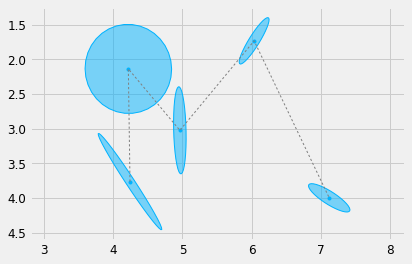
Lets load a sequence of \(5\) Gaussians for the letter "M"
#%%

import matplotlib.pyplot as plt

def load_gauss(path, scale=1.):
    Mu, Sigma = load_pkl(path)
    Mu *= scale
    Sigma *= scale**2
    return Mu, Sigma

Mu, Sigma = load_gauss('./m_1.pkl', scale=0.01)

# Plot it
plt.figure()
plot_gauss(Mu, Sigma)
plt.plot(Mu[0,:], Mu[1,:], ':', color=cfg.plan_color, linewidth=1.)
#plt.plot(Mu[0,:], Mu[1,:], 'ro')
plt_setup()
plt.show()
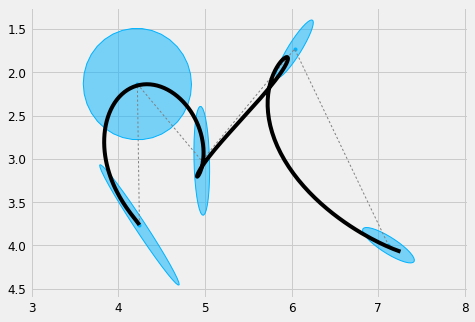
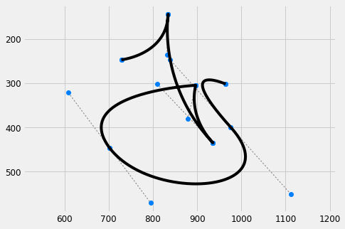
We can now generate a trajectory that tracks the Gaussians
#%%

order = 4
duration = Mu.shape[1]*0.2 # 0.2 seconds per state
sys = DynSys(order, dt=0.005)
n = sys.num_timesteps(duration)
endw = 1e10
r = 1e-10 # Regularisation
MuQ, Q = make_reference(Mu, Sigma, n, sys, reference=stepwise, end_weight=1e10)
x = iterative_mpc(sys, MuQ, Q, r=r)
y = sys.y(x)

# plot it
plt.figure(figsize=cfg.figsize)
plot_gauss(Mu, Sigma)
plt.plot(Mu[0,:], Mu[1,:], ':', color=cfg.plan_color, linewidth=1.)
plt.plot(y[0,:], y[1,:], 'k')
plt_setup()
plt.show()
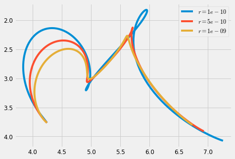
2.4.1 Regularisation
We can see the smoothing effect of the regularisation parameter \(r\) by increasing its value
#%%

plt.figure(figsize=cfg.figsize)
#plot_gauss(Mu, Sigma)
#plt.plot(Mu[0,:], Mu[1,:], ':', color=cfg.plan_color, linewidth=1.)

for r in [1e-10, 5e-10, 10e-10]: #, 15e-10]: #np.linspace(1e-10, 1e-13, 5):
    x = iterative_mpc(sys, MuQ, Q, r=r)
    y = sys.y(x)
    plt.plot(y[0,:], y[1,:], label='$r=' + str(r) + '$')
plt_setup()
plt.legend()
plt.show()
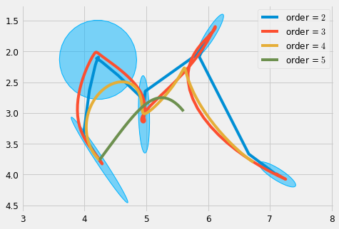
On the other hand, the behavior of this parameter will vary greatly across different system orders, which may be impractical for experimentation purposes.
#%%

plt.figure(figsize=cfg.figsize)

r = 1e-9
plot_gauss(Mu, Sigma)
for order in range(2, 6):
    sys = DynSys(order, dt=0.005)
    MuQ, Q = make_reference(Mu, Sigma, n, sys, reference=stepwise, end_weight=1e10) #1e-15) #0.)
    x = iterative_mpc(sys, MuQ, Q, r=r)
    y = sys.y(x)
    plt.plot(y[0,:], y[1,:], label='order = $' + str(order) + '$')
plt.legend()

plt_setup()
plt.savefig('r_scaling.pdf')
plt.show()
We can improve on this by specifying the regularisation through a maximum displacement parameter \(d\), which is can be computed based on the the low frequency gain of the system, where the frequency is chosen to be the period of an oscillatory motion between two targets. This can be computed with
#%%

def SHM_r(d, order, duration, m):
    ''' simple harmonic motion based scale factor,
        computes the control cost r in terms of maximum allowed displacement'''
    period = (duration/(m-1))
    omega = (2. * np.pi) / period
    return 1. / ((d * omega**order)**2)
and produces results that are more consistent across orders, and thus easier to control.
plt.figure(figsize=cfg.figsize)
d = 0.15
plot_gauss(Mu, Sigma)
for order in range(2, 6):
    sys = DynSys(order, dt=0.005)
    n = sys.num_timesteps(duration)
    MuQ, Q = make_reference(Mu, Sigma, n, sys, reference=stepwise, end_weight=1e10) #1e-15) #0.)
    r = SHM_r(d, order, duration, Mu.shape[1])
    x = iterative_mpc(sys, MuQ, Q, r=r)
    y = sys.y(x)
    plt.plot(y[0,:], y[1,:], label='order = $' + str(order) + '$')
plt.legend()

plt_setup()
plt.savefig('d_scaling.pdf')
plt.show()
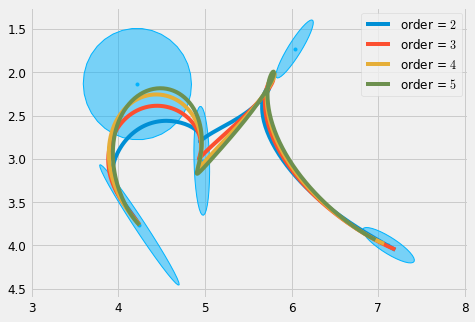
Note that in this case, decreasing the parameter \(d\) produces a smoothing effect on the trajectory.
2.5 Stochastic sampling
If we consider a Bayesian formulation of the batch version of the minimisation problem, we can interpret the generated trajectory as the center of a trajectory distribution [Calinon2016a]. This distribution defines a family of trajectories that can be stochastically sampled in order to generate variations that mimic the variability that would be seen in different traces made by a single user. While it would be possible to generate variations of a trajectory by perturbing the Gaussians or the optimisation parameters, this formulation allows a user to explicitly define which parts of the trajectory require higher precision and which ones have higher variability, while also defining the curvilinear evolution and smoothness of the trajectory.
The following code snippet extends the batch version of MPC to compute the covariance of the least squares estimate and to generate samples from the trajectory distribution.
#%%

from scipy.linalg import eigh

def largest_eigs(X, k):
    ''' Return k eigencomponents with decreasing eigenvalues'''
    N = X.shape[0]
    return eigh(X, eigvals=(N-k,N-1))

def stochastic_sample(x, Cov, mse, n_samples, n_eigs, sig=1.):
    ''' Generate samples from the trajectory distribution'''
    samps = []
    D, V  =  largest_eigs(Cov, n_eigs)
    D = np.real(np.diag(D))
    V = np.real(V)
    for i in range(n_samples):
         sigma =  np.sqrt(mse)*sig
         o = np.random.randn(n_eigs, 1)*sigma
         offset =  mul([ V, D**.5, o ])
         O = np.reshape( offset, (x.shape[1], x.shape[0])).T
         samp = x + O
         samps.append(samp)

    return samps
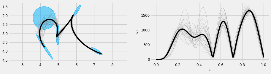
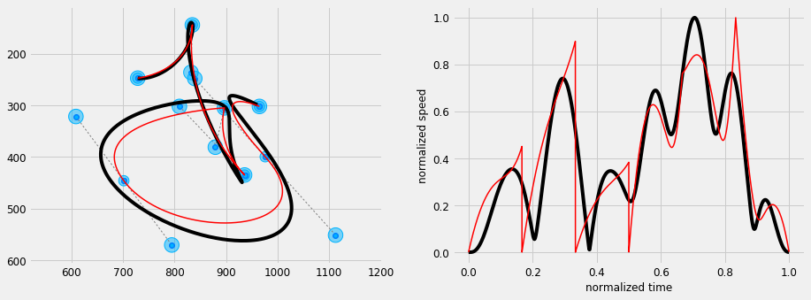
We can then stochastically sample this distribution in order to generate a possibly infinite number of variations over the mean trajectory.
#%%

import random
np.random.seed(2311)
order = 5

duration = Mu.shape[1]*0.2
sys = DynSys(order, dt=0.01)
n = sys.num_timesteps(duration)
MuQ, Q = make_reference(Mu, Sigma, n, sys, reference=stepwise, end_weight=1e10)
r = SHM_r(d, order, duration, Mu.shape[1])
x, Cov, mse = batch_mpc(sys, MuQ, Q, r=r, compute_covariance=True)

samps = stochastic_sample(x, Cov, mse, 40, 7, sig=2.5)
samps = [sys.y(samp) for samp in samps]
#x = iterative_mpc(sys, MuQ, Q, r=r)

y = sys.y(x)

# time
T = np.linspace(0, duration, n)
cfg.plan_color = [0.5, 0.5, 0.5]
plt.figure(figsize=(cfg.fig_w*2.0, cfg.fig_h*0.7))
plt.subplot(1, 2, 1)
#plt.title('Trajectory samples')
plot_gauss(Mu, Sigma) # Note this function def is hidden for saving space
#plt.plot(Mu[0,:], Mu[1,:], ':', color=cfg.plan_color)
np.random.seed(32)
rand_grey = lambda: np.ones(3) * np.random.uniform(0.1, 0.9)
for s in samps:
    plt.plot(s[0,:], s[1,:], 'm', label='samples', linewidth=0.2, color=rand_grey() )
plt.plot(y[0,:], y[1,:], 'k', label='mean trajectory')
plt_setup()
#plt.legend()

plt.subplot(1, 2, 2)
#plt.title('Speed')
np.random.seed(32)
for s in samps:
    S = norm(deriv(s*100, sys.dt, 1))
    plt.plot(np.linspace(0, duration, S.size), S, 'm', linewidth=0.2, color=rand_grey())
S = norm(deriv(y*100, sys.dt, 1))
plt.plot(np.linspace(0, duration, S.size), S, 'k')
plt.gca().set_xlabel('$t$')
plt.gca().set_ylabel(r'$\left\| \dot{x} \right\|$')
plt.savefig('stochastic_n.pdf')
plt.show()
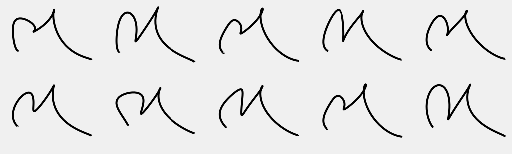
And plot some random samples
nrows = 2
ncols = 5
n_samps = nrows*ncols
figw = 1.6
plt.figure(figsize=(figw*n_samps, 0.3*figw*n_samps))
random.seed(72)
random.seed(911972)

for i in range(n_samps):
    plt.subplot(nrows, ncols, i+1)
    s = random.choice(samps)
    plt.plot(s[0,:], s[1,:], 'k')
    plt_setup(False)
plt.savefig('stochastic_n_samples.pdf')
plt.show()
2.6 Bezier curve approximation
We demonstrate how Gaussians with isotropic covariance can be used for computing approximations of Bezier curves [4].
Lets first define some code to load Bezier paths from a SVG file, using the svgpathtools package.
#%%

import svgpathtools as svg

def to_pt(c):
    ''' convert complex number to np vector'''
    return np.array([c.real, c.imag])

def to_bezier(piece):
    ''' convert a line or Bezier segment to control points'''
    one3d = 1./3
    if type(piece)==svg.path.Line:
        a, b = to_pt(piece.start), to_pt(piece.end)
        return [a, a+(b-a)*one3d, b+(a-b)*one3d, b]
    elif type(piece)==svg.path.CubicBezier:
        return [to_pt(piece.start),
                to_pt(piece.control1),
                to_pt(piece.control2),
                to_pt(piece.end)]
    raise ValueError

def path_to_bezier(path):
    ''' convert SVG path to a Bezier control points'''
    pieces = [to_bezier(piece) for piece in path]
    bezier = [pieces[0][0]] + sum([piece[1:] for piece in pieces],[])
    return np.vstack(bezier).T

def svg_to_beziers(path):
    ''' Load Bezier curves from a SVG file'''
    paths, attributes = svg.svg2paths(path)
    beziers = [path_to_bezier(path) for path in paths]
    return beziers
And some code to sample a piecewise Bezier curve for plotting.
def num_control_points(n_bezier):
    return 1 + 3*n_bezier

def num_bezier(n_ctrl):
    return int((n_ctrl - 1) / 3)

def num_targets(n_ctrl):
    return num_bezier(n_ctrl)-1

def bezier_piecewise(Cp, subd=1000):
    ''' sample a piecewise Bezier curve given a sequence of control points'''
    num = num_bezier(Cp.shape[1])
    X = []
    for i in range(num):
        P = Cp[:,i*3:i*3+4].T
        t = np.linspace(0, 1., subd)[:-1].reshape(-1,1)
        t = np.hstack([t, t])
        Y = (1.0-t)**3 * P[0] + 3*(1.0-t)**2 * t * P[1] + 3*(1.0-t)* t**2 * P[2] + t**3 * P[3]
        X += [Y.T]
    X = np.hstack(X)
    return X

def plot_control_polygon(Cp):
    n_bezier = num_bezier(Cp.shape[1])
    for i in range(n_bezier):
        cp = cp = Cp[:,i*3:i*3+4]
        plt.plot(cp[0,0:2], cp[1,0:2], ':', color=cfg.plan_color, linewidth=1.)
        plt.plot(cp[0,2:], cp[1,2:], ':', color=cfg.plan_color, linewidth=1.)
        plt.plot(cp[0,:], cp[1,:], 'o', color=[0, 0.5, 1.])

Cp = svg_to_beziers('./a.svg')[0]
yb = bezier_piecewise(Cp)

plt.figure(figsize=cfg.figsize)
plot_control_polygon(Cp)
plt.plot(yb[0,:], yb[1,:], 'k')
plt_setup()
plt.show()
It turns out that we can closely imitate the Bezier curve, using MPC and a stepwise reference with isotropic Gaussians. To achieve a similar curve, it is necessary to adjust some parameters, such as the maximum displacement \(d\) and the relative variance of the Gaussians corresponding with internal control points.
#%%

def mpc_bezier_stepwise(Cp, order, ctrl_ratio, max_d, dt=0.005):
    ''' Mimic a Bezier curve with isotropic Gaussians and a stepwise tracking reference'''
    sys = DynSys(order, dt=dt)

    m = Cp.shape[1]

    T = 0.25 * m #1.0*num_bezier(m)
    n = int(T / sys.dt)

    Mu = np.zeros((2,m))
    Sigma = np.zeros((2,2,m))

    for i in range(num_bezier(m)):

        p1,p2,p3,p4 = [Cp[:,j+i*3] for j in range(4)]

        d = (p1 - p2 + p4 - p3)/2

        dr = 0.0
        Mu[:,i*3] = p1
        Mu[:,i*3+3] = p4
        Mu[:,i*3+1] = p2 + d*dr #- d1*dr
        Mu[:,i*3+2] =  p3 + d*dr #- d2*dr

        sigma = np.eye(2)
        Sigma[:,:,i*3]   = sigma
        Sigma[:,:,i*3+1] = np.eye(2)*ctrl_ratio
        Sigma[:,:,i*3+2] = np.eye(2)*ctrl_ratio
        Sigma[:,:,i*3+3] = sigma

    MuQ, Q = make_reference(Mu, Sigma, n, sys, reference=stepwise, end_weight=1e10)

    r = SHM_r(max_d, order, T, m)

    x = iterative_mpc(sys, MuQ, Q, r=r)
    y = sys.y(x)
    return y, Mu, Sigma

plt.figure(figsize=(cfg.fig_w*2, cfg.fig_h))
# Plot Bezier and MPC overlaid
plt.subplot(1, 2, 1)
plot_control_polygon(Cp)
y, Mu, Sigma = mpc_bezier_stepwise(Cp,
                                   order=4,
                                   ctrl_ratio=2.0,
                                   max_d=0.01)
plot_gauss(Mu, Sigma, scale=100.)
plt.plot(y[0,:], y[1,:], 'k', label='MPC')
plt.plot(yb[0,:], yb[1,:], 'r', linewidth=1.5, label='Bezier')
plt_setup()

plt.subplot(1, 2, 2)
# compute speed and normalize
S = norm(deriv(y, 0.01, 1))
Sb = norm(deriv(yb, 0.01, 1))
S = S/np.max(S)
Sb = Sb/np.max(Sb)
plt.plot(np.linspace(0, 1., S.shape[0]), S, 'k')
plt.plot(np.linspace(0, 1., Sb.shape[0]), Sb, 'r', linewidth=1.5)
plt.gca().set_xlabel('normalized time')
plt.gca().set_ylabel('normalized speed')
plt.show()
This formulation can be useful to interactively edit a trajectory with an interface similar to the one offered by Bezier curves, while guaranteeing a smooth trajectory regardless of the positioning of control points. While this approach may not be ideal for a design oriented application, where a high precision is desirable, it can come handy for applications that require the simulation of a hand-drawn trace, where trajectory smoothness is more important.
2.7 Interpolation with MPC
The same optimisation method can be used to generate interpolating trajectories (passing through via-points). To do so, we define a sparse reference, in which a desired state in only specified in correspondence with its desired time step. For the case in which the time occurrence of the states is equally spaced in time we can define a new reference function:
#%%
def via_points(m, n):
    ''' Get via-point reference indices
    returns target indices, and corresponding time steps in reference for each index'''
    a, b = 0., n-1
    return range(m), [ int(a + i*(b-a)/(m-1)) for i in range(m) ]

# For 30 time steps and 3 via points:
Ts = -np.ones(30).astype(int)
I, T = via_points(3, 30)
Ts[T] = I

plt.figure(figsize=(14,0.5))
plt.gca().pcolormesh([[ float(t)/3+0.5 if t >= 0 else 0 for t in Ts]], cmap='Spectral', edgecolor='k', vmin=-1., vmax=1.)
for i, t in enumerate(Ts):
    if t >= 0:
        plt.text(0.4 + i, 0.5,str(t))
plt.axis('off')
plt.show()

We then express the penality of deviating from a desired state with an indentity covariance matrix, which corresponds to a cost given by the Euclidean distance to a target.
def load_and_interpolate(path, order, stroke_duration=0.3, scale=1./100000):
    Mu, Sigma = load_gauss(path, scale=scale)
    duration = Mu.shape[1]*stroke_duration
    sys = DynSys(order, dt=0.005)
    n = sys.num_timesteps(duration)

    endw = 1.
    r = 1e-10

    MuQ, Q = make_reference(Mu, Sigma, n, sys, reference=via_points, end_weight=endw) #1e-15) #0.)
    x = iterative_mpc(sys, MuQ, Q, r=r)

    return Mu, Sigma, sys.y(x)

dt = 0.005
orders = range(2,6)

plt.figure(figsize=(cfg.fig_w*len(orders), cfg.fig_h))
for i,order in enumerate(orders):
    plt.subplot(1, len(orders), i+1)
    plt.title('$n=' + str(order) + '$')
    Mu, Sigma, x = load_and_interpolate('e.pkl', order)
    plt.plot(Mu[0,:], Mu[1,:], ':', color=cfg.plan_color, linewidth=1.)
    plt.plot(Mu[0,:], Mu[1,:], 'o', color=[0,0.5,1.], linewidth=1.)
    plt.plot(x[0,:], x[1,:], 'k')
    plt_setup()

plt.show()
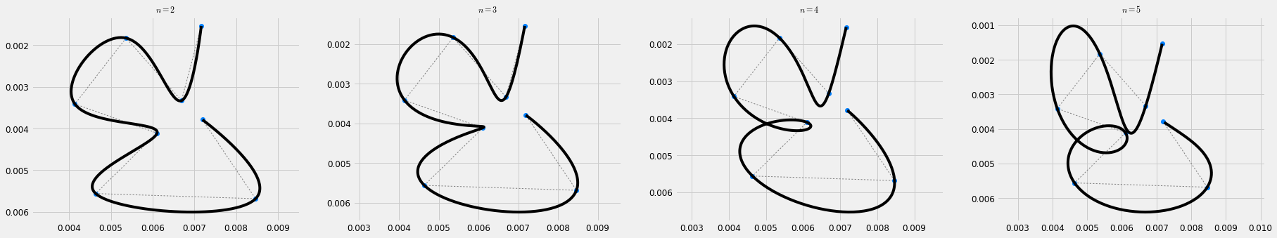
The resulting trajectories interpolate the given sequence of targets, while minimising the squared norm of control command. While this is similar to the trajectory formation models known as Minimum Square Derivative (MSD) methods (e.g. Minimum Jerk (MJ) [flash1985coordination] or Minimum Snap (MS) [Edelman1987] ), here we perform a simplifying assumption of a perfectly equal spacing in time between via-points and accordingly an equal duration of the corresponding trajectory segments. On the other hand, the MSD methods predict an approximatley but no equal duration of the trajectory segments, which is predicted by the models as a result of the optimisation. While we leave a more accurate computation of the timing aspects of the trajectory for further steps of the study, we demonstrate how this can be achieved for a MJ trajectory with one via point by using the method described by Flash and Hogan in [flash1985coordination].
The MJ trajectory has a closed form solution given by a polynomial of order \(5\), which can be computed with the following function
#%%

def min_jerk_via( x0,x1,xf, t, t1, tf ):
    tau1 = t1 / tf
    tau = t / tf
    tf5 = tf**5
    ta2 = tau**2
    ta3 = tau**3
    ta4 = tau**4
    ta5 = tau**5
    ta1_2 = tau1**2
    ta1_3 = tau1**3
    ta1_4 = tau1**4
    ta1_5 = tau1**5

    c = ( (1 / (tf5*ta1_2*(1 - tau1)**5)) * ((xf - x0)*(300.*ta1_5 - 1200.*ta1_4 + 1600.*ta1_3)
        + ta1_2*(-720.*xf + 120.*x1 + 600.*x0)
            + (x0 - x1)*(300*tau1 - 200)))

    p = ( (1 / (tf5*ta1_5*(1 - tau1)**5)) * ((xf - x0)*(120*ta1_5
            - 300.*ta1_4 + 200.*ta1_3) - 20*(x1 - x0)))

    x = ((tf5/720.) * (p*(ta1_4*(15.*ta4 - 30.*ta3)
    + ta1_3*(80.*ta3 - 30.*ta4) - 60.*ta3*ta1_2 + 30.*ta4*tau1 - 6.*ta5)
                  + c*(15.*ta4 - 10.*ta3 - 6.*ta5)) + x0)
    if t > t1:
        x = x + p * ( tf5 * (tau - tau1)**5 ) / 120.
    return x
The time occurrence of the via point is given by the real root of a \(9\mathrm{th}\) order polynomial, which we use SymPy to compute
import sympy as sym
def solve_tau1(X):
    vals = sym.symbols('x_0, y_0, x_1, y_1, x_f, y_f', real=True)
    x_0, y_0, x_1, y_1, x_f, y_f = vals
    v = [X[0,0], X[1,0], X[0,1], X[1,1], X[0,2], X[1,2]]
    tau_1 = sym.symbols('tau_1', real=True)
    # quite a beast...
    poly = 6*tau_1**9*x_0**2 - 12*tau_1**9*x_0*x_f + 6*tau_1**9*x_f**2 + 6*tau_1**9*y_0**2 \
           - 12*tau_1**9*y_0*y_f + 6*tau_1**9*y_f**2 - 27*tau_1**8*x_0**2 + 54*tau_1**8*x_0*x_f \
           - 27*tau_1**8*x_f**2 - 27*tau_1**8*y_0**2 + 54*tau_1**8*y_0*y_f - 27*tau_1**8*y_f**2 \
           + 40*tau_1**7*x_0**2 - 80*tau_1**7*x_0*x_f + 40*tau_1**7*x_f**2 + 40*tau_1**7*y_0**2 \
           - 80*tau_1**7*y_0*y_f + 40*tau_1**7*y_f**2 - 8*tau_1**6*x_0**2 - 12*tau_1**6*x_0*x_1 \
           + 28*tau_1**6*x_0*x_f + 12*tau_1**6*x_1*x_f - 20*tau_1**6*x_f**2 - 8*tau_1**6*y_0**2 \
           - 12*tau_1**6*y_0*y_1 + 28*tau_1**6*y_0*y_f + 12*tau_1**6*y_1*y_f - 20*tau_1**6*y_f**2 \
           - 36*tau_1**5*x_0**2 + 36*tau_1**5*x_0*x_1 + 36*tau_1**5*x_0*x_f - 36*tau_1**5*x_1*x_f \
           - 36*tau_1**5*y_0**2 + 36*tau_1**5*y_0*y_1 + 36*tau_1**5*y_0*y_f - 36*tau_1**5*y_1*y_f \
           + 34*tau_1**4*x_0**2 - 34*tau_1**4*x_0*x_1 - 34*tau_1**4*x_0*x_f + 34*tau_1**4*x_1*x_f \
           + 34*tau_1**4*y_0**2 - 34*tau_1**4*y_0*y_1 - 34*tau_1**4*y_0*y_f + 34*tau_1**4*y_1*y_f \
           - 8*tau_1**3*x_0**2 + 8*tau_1**3*x_0*x_1 + 8*tau_1**3*x_0*x_f - 8*tau_1**3*x_1*x_f \
           - 8*tau_1**3*y_0**2 + 8*tau_1**3*y_0*y_1 + 8*tau_1**3*y_0*y_f - 8*tau_1**3*y_1*y_f \
           - 2*tau_1*x_0**2 + 4*tau_1*x_0*x_1 - 2*tau_1*x_1**2 - 2*tau_1*y_0**2 + 4*tau_1*y_0*y_1 \
           - 2*tau_1*y_1**2 + x_0**2 - 2*x_0*x_1 + x_1**2 + y_0**2 - 2*y_0*y_1 + y_1**2
    eval_poly = poly.subs(dict(zip(vals,v)))
    expr = (sym.expand(eval_poly.as_expr()))
    realroot = sym.nsolve(expr, 0.5)
    return float(realroot)

def via_points_tau1(m, n, tau_1):
    ''' Get via-point reference indices
    returns target indices, and corresponding time steps in reference for each index'''
    a, b = 0., n-1
    I = range(m)
    t1_n = int(tau_1*n)
    T = [0, t1_n, n-1]
    return I, T #range(m), [ int(a + i*(b-a)/(m-1)) for i in range(m) ]
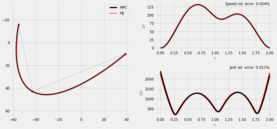
We then can compare the MPC solution to the original closed form solution
def rel_err(x, x_hat):
    '''Relative error [0-1]'''
    e = (np.sum(np.abs(x-x_hat)) / np.sum(x_hat)) / len(x_hat)
    return e


sys = DynSys(3, 0.005)
duration = 2.
n = sys.num_timesteps(duration)

# MPC trajectory
plt.rc('text', usetex = False)
m = 3
np.random.seed(123)
Mu = np.floor(np.random.uniform(-100, 100, size=(2, m)))
Sigma = np.dstack([np.eye(2,2) for i in range(m)])

# Solve for via point relative time
tau_1 = solve_tau1(Mu)

MuQ, Q = make_reference(Mu, Sigma, n, sys, reference=lambda m,n: via_points_tau1(m, n, tau_1), end_weight=1.)
x = iterative_mpc(sys, MuQ, Q, r=1e-10)
y = sys.y(x)

# time steps
T = np.linspace(0, duration, n)

# Minimum jerk trajectory
yj = np.array([ min_jerk_via(Mu[:,0], Mu[:,1], Mu[:,2], t, tau_1*duration, duration) for t in T]).T

plt.figure(figsize=(cfg.fig_w*2, 1.3*cfg.fig_h)) #(15,5))
vmargin = 0.4
plt.subplots_adjust(hspace=vmargin) #, top=vmargin+2.)
plt.subplot2grid((2, 2), (0,0), rowspan=2)
plt.plot(Mu[0,:], Mu[1,:], ':', color=cfg.plan_color, linewidth=1.)
plt.plot(Mu[0,:], Mu[1,:], 'o', color=[0,0.5,1.])
plt.plot(Mu[0,0:1], Mu[1,0:1], 'ro') #, color=[0,0.5,1.])
plt.plot(y[0,:], y[1,:], 'k', label='MPC')
plt.plot(yj[0,:], yj[1,:], 'r', label='MJ', linewidth=1.5)

plt_setup()
plt.legend()

# Speed error
plt.subplot2grid((2, 2), (0,1))
#plt.title('Speed')
S = norm(deriv(y, sys.dt, 1))
Sj = norm(deriv(yj, sys.dt, 1))
# size hack for time
T = np.linspace(0, duration, len(Sj))
err = rel_err(S, Sj)
errstr = ('%.3f'%(err*100)) + '%'
plt.plot(T, S, 'k')
plt.plot(T, Sj, 'r', linewidth=1.5)
plt.text(2.0, 130, 'Speed rel. error: ' + errstr, horizontalalignment='right')
plt.gca().set_xlabel('$t$')
plt.gca().set_ylabel(r'$\left\| \dot{x} \right\|$')

# Jerk error
plt.subplot2grid((2, 2), (1,1))
#plt.title('Jerk')
S = norm(deriv(y, sys.dt, 3))[1:]
Sj = norm(deriv(yj, sys.dt, 3))[1:]
# size hack for time
T = np.linspace(0, duration, len(Sj))
err = rel_err(S, Sj)
errstr = ('%.3f'%(err*100)) + '%'
plt.plot(T, Sj, 'r')
plt.plot(T, S, 'k')
plt.text(2., 2500.0, 'Jerk rel. error: ' + errstr, horizontalalignment='right')
plt.gca().set_xlabel(r'$t$')
plt.gca().set_ylabel(r'$\left\| \dot\ddot{x} \right\|$')

# Save and show
plt.savefig('mj.pdf')
plt.show()
3 Stylisation and Semi-tied Gaussians
If we look at the proposed optimal control formulation of trajectories for the case of letter forms, we can consider different stylisations of a letter with a bi level representation, in which the sequence of targets defines an overall structure, and different trajectories that follow Gaussians placed in correspondence with the targets define different stylisations of the same structure. This representation is similar to the one proposed by semiotician William C. Watt [Watt1988]. Watt used formal grammars to study the evolution of written letters in history through two complemtary descriptors: one iconic that describes the letter form as a symbol, and one kinemic that describes the movements used to produce the letter when writing. We can exploit a similar framework to generate different stylisation of letters defined as sparse sequneces of targets.
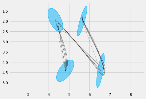
As an example we can take the target description of a letter "N". We can for example generate different stylisations of the letter by varying the maximum displacement parameter \(d\), where a lower value of \(d\) will produce smoother trajectories. Watt calls this process "facilitation", i.e. the tendency to produce a letter form with a reduced effort, whic results in smoother traces.
#%%
Mu, Sigma = load_gauss('./n.pkl', scale=0.01)

order = 5
duration = Mu.shape[1]*0.2 # 0.2 seconds per state
sys = DynSys(order, dt=0.005)
n = sys.num_timesteps(duration)
endw = 1e10

plt.figure(figsize=cfg.figsize)
plot_gauss(Mu, Sigma)
plt.plot(Mu[0,:], Mu[1,:], ':', color=cfg.plan_color, linewidth=1.)

for d in np.linspace(0.2, 0.6, 4):
  r = SHM_r(d, order, duration, Mu.shape[1])
  MuQ, Q = make_reference(Mu, Sigma, n, sys, reference=stepwise, end_weight=1e10) #1e-15) #0.)
  x = iterative_mpc(sys, MuQ, Q, r=r)
  y = sys.y(x)
  plt.plot(y[0,:], y[1,:], 'k', linewidth=0.5)
plt_setup()
plt.show()
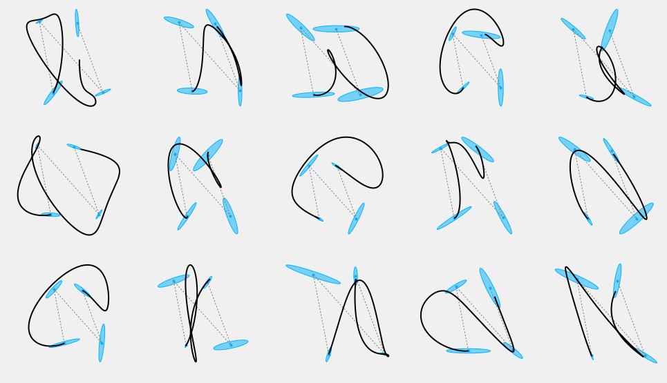
Other stylistic variations can be produced by varying other parameters, such as the orientation and scale of the covariances corresponding with each target. If we try to randomly generate covariances for each target, we can see that this process may be actually hard to control and often produce unpredictable results:
#%%
def make_sigma(theta, scale):
    ''' Builds a 2d covariance with a rotation and scale'''
    scale=np.array(scale)

    # rotation matrix
    Phi = np.eye(2, 2)
    ct = np.cos(theta)
    st = np.sin(theta)
    Phi[0,0], Phi[0,1] = ct, -st
    Phi[1,0], Phi[1,1] = st, ct

    # scale matrix
    S = np.diag(scale*scale)
    return mul([Phi, S, Phi.T])

# Fix the seed for demonstration purposes
np.random.seed(326)
n_rows = 3
n_cols = 5
nsamples = n_rows*n_cols
plt.figure(figsize=(3*n_cols, 3*n_rows))

for i in range(nsamples):
    plt.subplot(n_rows, n_cols, i+1)
    Sigma2 = np.array(Sigma)
    for j in range(Mu.shape[1]):
        s = np.random.uniform(0.1, 0.9)
        Sigma2[:,:,j] = make_sigma(np.random.uniform(-np.pi, np.pi),
                                    [s, s*np.random.uniform(0.1, 0.2)]) #np.random.uniform(0.02, 0.5, 2))

    plot_gauss(Mu, Sigma2)
    plt.plot(Mu[0,:], Mu[1,:], ':', color=cfg.plan_color, linewidth=1.)

    r = SHM_r(0.3, order, duration, Mu.shape[1])
    MuQ, Q = make_reference(Mu, Sigma2, n, sys, reference=stepwise, end_weight=1e10) #1e-15) #0.)
    x = iterative_mpc(sys, MuQ, Q, r=r)
    y = sys.y(x)
    plt.plot(y[0,:], y[1,:], 'k', linewidth=2)
    plt_setup(axis=False)
plt.show()
One way to overcome this problem and maintain a greater control over the results, is to force a shared orientation for all the covariance ellipsoids
n_rows = 3
n_cols = 5
nsamples = n_rows*n_cols
plt.figure(figsize=(3*n_cols, 3*n_rows))
Theta = np.random.uniform(-np.pi, np.pi, nsamples)
np.random.seed(326)
for i in range(nsamples):
    plt.subplot(n_rows, n_cols, i+1)
    Sigma2 = np.array(Sigma)

    for j in range(Mu.shape[1]):
        s = np.random.uniform(0.1, 0.9)
        np.random.uniform(-np.pi, np.pi) # Just to keep the same seed
        Sigma2[:,:,j] = make_sigma(Theta[i],
                                   [s, s*np.random.uniform(0.1, 0.2)]) #np.random.uniform(0.02, 0.5, 2))

    plot_gauss(Mu, Sigma2)
    plt.plot(Mu[0,:], Mu[1,:], ':', color=cfg.plan_color, linewidth=1.)

    r = SHM_r(0.3, order, duration, Mu.shape[1])
    MuQ, Q = make_reference(Mu, Sigma2, n, sys, reference=stepwise, end_weight=1e10) #1e-15) #0.)
    x = iterative_mpc(sys, MuQ, Q, r=r)
    y = sys.y(x)
    plt.plot(y[0,:], y[1,:], 'k', linewidth=2)
    plt_setup(axis=False)
plt.show()
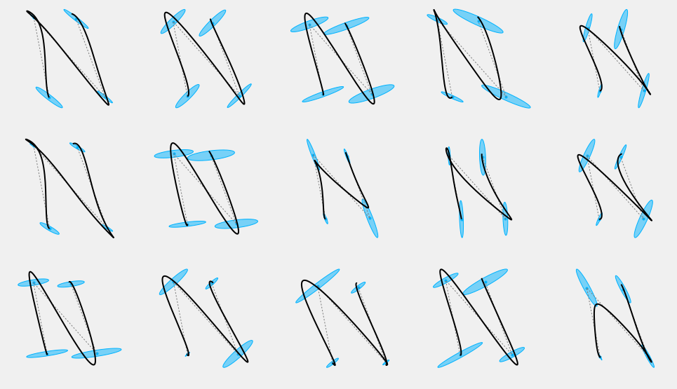
Different orientations give consistently different stylisations of the same sequence of targets.
This form of covariance formulation is known as semi-tied, and has been shown to describe well coordination patterns in human movements [Tanwani2016,Avella2003]. Interestingly, an examination of the handwriting synthesis literature suggests another possible physical interpretation of this result. It has been proposed that handwriting evolves in an "oblique" coordinate system [Dooijes1983,Maarse1987,Meulenbroek1991] which can be approximated via a shear (linear) transformation.
Bibliography
- [Calinon2016] Calinon, A tutorial on task-parameterized movement learning and retrieval, Intelligent Service Robotics, 9(1), 1-29 (2016).
- [Todorov2004] Todorov, Optimality principles in sensorimotor control, Nature neuroscience, 7(9), 907-915 (2004).
- [Flash2005] Flash & Hochner, Motor primitives in vertebrates and invertebrates, Current opinion in neurobiology, 15(6), 660-6 (2005).
- [Egerstedt2004] Egerstedt, Martin & others, A note on the connection between Bezier curves and linear optimal control, IEEE transactions on automatic control, 49(10), 1728-1731 (2004).
- [flash1985coordination] Flash & Hogan, The coordination of arm movements, Journal of Neuroscience, 5(7), 1688-1703 (1985).
- [Edelman1987] Edelman & Flash, A model of handwriting, Biological cybernetics, 57(1-2), 25-36 (1987).
- [Dingwell2004] Dingwell, Mah & Mussa-Ivaldi, Experimentally confirmed mathematical model for human control of a non-rigid object, Journal of Neurophysiology, 91(3), 1158-1170 (2004).
- [freedberg2007motion] Freedberg & Gallese, Motion, emotion and empathy in esthetic experience, Trends in cognitive sciences, 11(5), 197-203 (2007).
- [pignocchi2010] Pignocchi, How the Intentions of the Draftsman Shape Perception of a Drawing, Consciousness and Cognition, 19(4), 887-898 (2010).
- [DePreester2014] De Preester & Tsakiris, Sensitivity to differences in the motor origin of drawings: from human to robot, PloS one, 9(7), e102318 (2014).
- [Calinon2016a] Calinon, Stochastic learning and control in multiple coordinate systems, in in: Intl Workshop on Human-Friendly Robotics, edited by (2016)
- [Watt1988] @InCollectionWatt1988, author = Watt, William C, title = Canons of alphabetic change, booktitle = The alphabet and the brain, publisher = Springer, year = 1988, pages = 122-152,
- [Tanwani2016] Tanwani & Calinon, Learning Robot Manipulation Tasks With Task-Parameterized Semitied Hidden Semi-Markov Model, IEEE Robotics and Automation Letters, 1(1), 235-242 (2016).
- [Avella2003] d'Avella, Saltiel & Bizzi, Combinations of muscle synergies in the construction of a natural motor behavior, Nature neuroscience, 6(3), 300-308 (2003).
- [Dooijes1983] Dooijes, Analysis of handwriting movements, Acta Psychologica, 54(1), 99-114 (1983).
- [Maarse1987] Maarse, The study of handwriting movement: Peripheral models and signal processing techniques, Lisse [etc.]: Swets & Zeitlinger (1987).
- [Meulenbroek1991] Meulenbroek & Thomassen, Stroke-direction preferences in drawing and handwriting, Human Movement Science, 10(2-3), 247-270 (1991).
Created: 2017-05-13 Sat 21:11