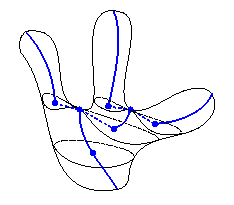
An LSD (bold blue lines) of an object defined by the centroids
of the connected components of the level sets (thin lines) of a given
function.
Joints between LSD branches are indicated as dashed blue lines.
Last update: Feb. 18, 2004
Publications by INRIA projects on 3D Shape Analysis & Metamorphosis :
BibTeX references.
URL's:
Francis
Lazarus and Anne Verroust
Rapport de recherche de l'INRIA- Rocquencourt
no. RR-3546
Projet : SYNTIM - 22 pages - Novembre 1998
Proceedings of the fifth ACM symposium on Solid
modeling and applications
Ann Arbor, Michigan, United States
Pages: 130 - 140, 1999
Shape descriptors and feature-based representations are of primary interests in the area of solid modeling. They allow us for easier storage, recognition and general treatments of objects. Axial structures such as skeletons are popular shape descriptors which have been widely studied. Most of the studies focus on a particular type of skeleton called the Medial Axis. Medial Axes can be extracted from discrete volumetric data as well as boundary-based representations. In the later case, however, no algorithm is known to perform well and accurately.
We propose a new paradigm for constructing 1D axial structures associated with a polyhedral object. These structures, called the level set diagrams, are associated with scalar functions defined over the set of vertices of a polyhedron. We study in details the level set diagram associated with the shortest path distance to a source point. This particular association fits nicely into a theoretical framework and presents interesting properties for the purpose of shape description.
Keywords : Skeleton, Cylindrical decomposition, Euler formula, Dijkstra's algorithm.
New paradigm for constructing 1D axial structures, the Level Set Diagram (LSD) associated to a polyhedral object. It capture the overall shape (geometry) as well as the topology of an object. It can be used for deformation and animation purposes. It is much simpler than algorithms that compute the Medial Axes of polyhedral objects. The latter start with adding points on the object's boundary and compute their Delaunay triangulation. The resulting Medial axes need to be prunned.
LSDs are simple 1D graphs which relate to the level sets of scalar function defined over the vertices of a polyhedral surface. The points of an LSD correspond to "average points" associated with the connected components of the level sets of a given scalar function, f . Branches of the LSD are connected through virtual links with critical vertices of the surface P of the object.

An LSD (bold blue lines) of an object defined by the centroids
of the connected components of the level sets (thin lines) of a given
function.
Joints between LSD branches are indicated as dashed blue lines.
The function f is often taken to be the height function relatively to a given orientation of the object. This is particularly meaningful for terrain data as critical points of f (i.e., points where the gradient is null) correspond to peaks, pits & passes. However, it is proposed that the shortest path distance to a source point is a often a better choice of function, especially for describing the geometry of tubular and branching objects.
Only LSDs of triangulated polyhedra, P, are considered here. Let f be a function over the vertices of P (v1, ..., vn) s.t. 2 adjacent vertices are given 2 different values. All that is needed is to tell which of any such 2 adjacent vertices gets the smaller values (ordering); vertices who get identical values can be ordered arbitrarily.
f(vi) < l < f(vj) < f(vk)
or
f(vi) < f(vj) < l < f(vk)
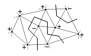
A triangulation with its cross-adjency graph (bold lines) for a given
level set l.
Vertices with values greater (smaller) than l are marked with a
"+" (a "-").


Segment (pij(l) pik(l)) is the geometric realization
of the cross-face (vi, vj, vk) .
Indf(v) = 1 - 0.5 Sgcf(v)

Where X(P) = nV - nE + nF, is the classic Euler characteristic of P, in terms of the number of vertices, edges & faces of P.
In Morse theory, one may speak of the index of a critical point of a gradient vector field , i.e. at a point where the vector field is null: one measures the number of revolutions made by the vector field while turning around that point. The analogy with the above vertex index can be made where one first orient the edges according to the f-values of their endpoints. This orientation corresponds to the gradient of f along the edges.
A triangle must have 2 edges oriented the same way and 3rd one oriented the other way. Then, in each triangle of P, we can draw a continuous vector field, s.t. the direction of the vector field on the boundary agrres with the orientation of its edges. The vertices of P are the critical points of this (induced) vector field. The (Morse) index of this critical points corresponds the vertex index introduced above.
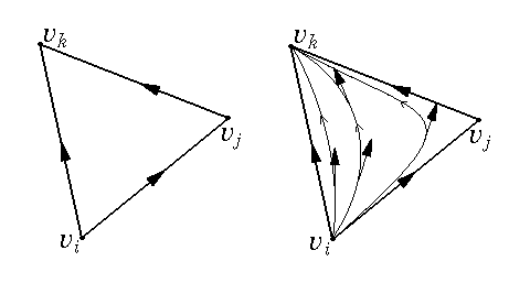
LHS: Orientation of the triangle edges induced by f (f(vi)
< f(vj) < f(vk)).
RHS: Tangent vectors of the oriented curves defined thru a compatible
vector field.
The vertex index thus describes how the level set realization, C(l), is modified around any given vertex, v, as the level l is raised from f(v) - e to f(v) + e , for a sufficiently small e. Note: This is similar to the construction of Dupin's indicatrix.
If Indf(v) is null, then the neighbors of v are partitioned into 2 connected sets {v- : f(v-) < f(v)}and {v+ : f(v+) > f(v)}.
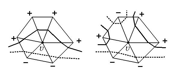
The ngb v in 2 different configurations s.t. Indf(v) = 0
on the left and -1 on the right.
Level set realization is shown for f either slightly below
(dotted curve) or above (plain bold curve) f(v).

2 configurations of a vertex with index -1. The number of connected
components
of the level sets increases on the LHS, while it decreases on the RHS.
While a choice of f as the height function is relevant for terrain-like surfaces (see Shinagawa et al.), a better choice to obtain level sets of tubular objects following their "natural" axes, is provided with the moving front of some flow emanating from the tip of a given tube. Such fronts corresponf to the geodesic distance to a tip of a tube.
As an approximation to the geodesic distance, it is proposed to compute the shortest path distance, ds, relatively to the graph induced by the edges of the polyhedron.
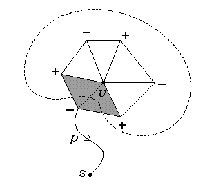
The path p : v -> s meets the realization
of any level set cycle (front)
containing one or more cross-faces (shaded area) incident to v once and
only once.
The tree structure of the LSD is recorded into a tree Ts(P) whose root, internal nodes and leaves are respectively the source s, the saddle vertices and the local maxima. The lines of Ts(P) link critical vertices and correspond to cylindrical parts of P.
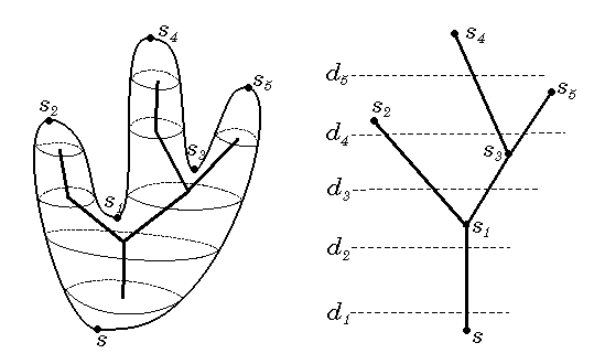
The LSD is an embedding of the tree Ts(P), here for 5 level sets
of ds.
Assumptions :
To construct the LSD, we need to sweep the level from zero to its maximum value max ds and compute "average" points of various level set cycles. Ts(P) provides an efficient tool to determine a starting edge in each cycle of any level set. For each line (si, sj) of Ts(P) we compute a starting cross-edge in any cycle contained in the associated cylindrical part, for a decreasing path (from sj ).
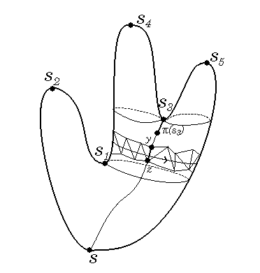
The pointer pi is used to find a starting cross-edge (y, z)
of a cycle contained in the cylindrical region between s1 & s3.
Ts(P) is constructed while traversing the adjency graph of P, where shortest path distance ds of the visited vertices, as well as the pointer pi to the preceding ngb on a shortest path, are computed. A priority queue with respect to distance is maintained (a la Dijkstra), which contains the adjacent vertices to already visited ones, but whose distance have not yet been fixed.
The complexity of each loop (cylindrical branch) reduces to Dijkstra's (O(n log n) using a Fibonacci heap, for a polyhedron made of n vertices). The total time spent splitting queues is bounded by ns.Lmax, where ns counts the number of saddles, and Lmax is the largest number of cross-edges in a level-set. Thus, the computation of Ts(P) requires time O(n log n + ns.Lmax).
The LSD is a geometric embedding of Ts(P).

|
|
Swan composed of 1728 faces & its LSD for 20 levels. |
2 source points & corresponding LSDs, almost identical. |
The LSD can handle self-intersections, which would not have been the case had a height function been used. Also, the Medial Axis Transform would fail (? not clear why ... ?).

Self-intersecting knot & its LSD.
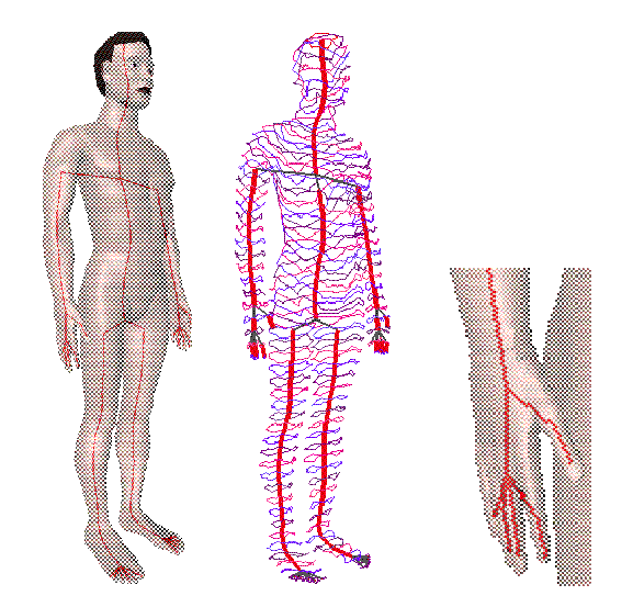
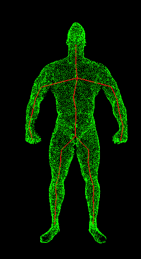
Man composed of 15000 faces with source point at top of the head.
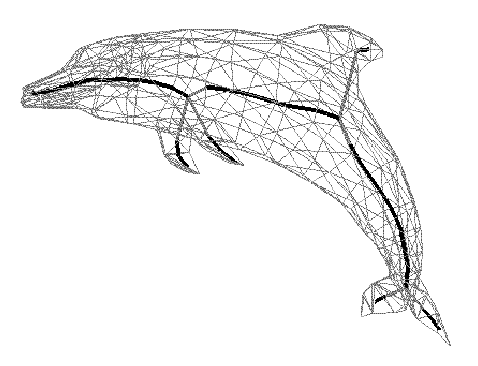
Dolphin composed of 563 faces and its LSD.
|
|
Horse composed of 22260 faces & its LSD. |
Bowl & LSDs before & after a bending of the LSD. |
N.B.: The LSD may lie outside of the object (see bowl above).
Anne
Verroust and Francis Lazarus
In Rapport de Recherche INRIA no 3250. September 1997.
Also published in
Shape
Modeling International '99. Aizu, Japan, March 1999.
Also published in
The
Visual Computer, Volume
16, Number 1, pages 15-25, 2000.
We introduce a method for the construction of skeletal curves from an unorganized collection of scattered data points lying on a surface. These curves may have a tree like structure to capture branching shapes such as blood vessels. The skeletal curves can be used for different applications ranging from surface reconstruction to object recognition. As an input, the algorithm takes a set of 3D points. It returns a set of curves arranged in a tree structure. The only interaction needed is the selection of a data point which represents the root of the tree. A neighborhood graph is constructed over the set of points to compute geodesic distances between the root point and the other points. Connected level sets of the distance map are then extracted and organized in a tree structure. The centers of these levels sets constitute the skeletal curves.
As opposed to most other approaches, which start from voxelized data to compute 3D medial axes, here one starts from an unorganized cloud of points sampled on a surface.
The computation of the axes is based on a cylindrical decomposition of the surface representing the set of 3D points. It is composed of 4 steps:

The main steps of the method.
The choice of k (level sets) is based on the number an locations of branches as well as the smoothness of the desired skeletal curves.
Each axis of the tree structure correspond to a tubular part of the surface. Their union forms a decomposition of the surface.

15 level sets computed on the geodesic graph of a femur and
corresponding axis.

Aorta

Blood vessels
Francis
Lazarus and Anne Verroust
Jour. of Visualization & Computer Animation, vol.8(3), pp.131-146,
1997.
Compute continuous shape transformations between polyhedral objects that are star-shaped around an axis (i.e., a generalised cylinder).
The user controls the global evolution of the deformation by specifying 2 corresponding skeletal structures in 3D, from which parametrizations of the sampling meshes are built.
The class of object considered, the star-shaped (cross-section) around an axis (3D axial curve), are split in 3 sheets: 2 hemispherical parts for the 2 end-points of the axis and 1 cylindrical part in between.
Many discretization aspects are treated by ad-hoc methods. For ecample, the recovery of "edge" (ridge) features of the original shape is done manually (it seems), which is deemed necessary to obtain reasonable cross-sections.
Francis
Lazarus, Sabine Coquillart and Pierre Jancene
In Computer-Aided Design, v.26(8), pp 607-613, August 1994.
Our current research efforts focus on providing more efficient and effective design methods for broadcast modeling systems. This paper is a revised version of Interactive axial deformations. It presents an interactive deformation technique called AxDf for Axial Deformations. Based on the paradigm of modeling tool, the Axial Deformations technique allows an easy specification of deformations that can be controlled with a 3D axis, such as bending, scaling, twisting and stretching. Moreover, AxDf can easily be combined with other existing deformation techniques.
Page created & maintained by Frederic Leymarie,
1998-2004.
Comments, suggestions, etc., mail to: leymarie@lems.brown.edu