
Figure 1 : Basic relationships between MAT point p, the
MA point p and
boundary footpoints q1 & q2.
The maximal ball definition of the MAT divided the MA points into three types: normal points, end points, and branch points. However, a better division is obtained by considering the tangent continuity of the MAT.
Two important results follow immediately from the theorem.
From these results, it is clear that a division of the MA into four types of points is more appropriate: normal points with a continuous tangent, normal points with a tangent discontinuity, end points, and branch points. Below we consider the conversion process for each of these four types of points.
Throughout this section we rely on the assumption that each curve of the MAT is parameterized with respect to arclength. We will also without further notice use the notation that p = (x, y, r) is a point on the MAT M of a simple object O and that p is its projection to the MA M. The MAT tangent at p is referred to as T while the tangent to M at p is given by T. Note that T is the projection of T to the xy-plane.
Figure 1 : Basic relationships between MAT point p, the
MA point p and
boundary footpoints q1 & q2.
The relationships shown in Figure 1 hold based on the following two lemmas.
These two lemmas can now be applied to compute the angle alpha between the MA tangent and the boundary normals:
Here l is the length of the T between p and w, that is, between the projection of p to the xy-plane and the intersection of the MAT tangent T with the xy-plane.
The basic technique for finding boundary points related to an MAT point p is to find the angle which the radial line connecting p to a related boundary point makes with the MA tangent at p. Related boundary points then must lie along those lines, distance r from p.
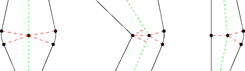
Figure 2 : From MA to Boundary points - joins:
doubly convex, concave-convex and simply convex.
For normal points with a continuous tangent, there are exactly two related boundary points, which are found as described above. Note that the boundary may have a concave corner which is related to multiple MAT points, but that the MAT can still be tangent continuous at those points. Such a situation is shown in the center of Figure 2. Here the boundary corner on the left side is related to MAT points on both sides of the corner in the MAT. The MAT is shown in green while some direction vectors are shown in red.
Figure 2 shows also the possible situations when the MAT has a tangent discontinuity at a normal point. By Theorem 1, at least one touching must be a finite contact. The sector(s) of the disc which are shared with the boundary are found by using the one-sided tangents along each approach to the point with the tangent discontinuity, and computing and angle alpha for each of these one-sided tangents. The region of the disc between pairs of related boundary points which are on the same side of the MA must be the boundary related to the MAT point.
The boundary related to a branch point is found analogously to that of a normal point with a tangent discontinuity, by computing an angle from each one-sided tangent to the MAT at the branch point. Again, if points in a region about the MAT do not match identically, then the segment of the disc between the two points in the region must be boundary related to the MAT point.
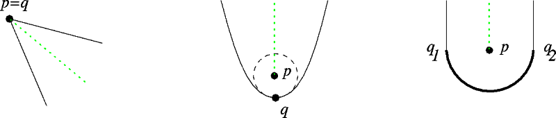
Figure 3 : The 3 possible types of end-points.
There are 3 situations possible for an end point, but each of them can be handled identically, by using the one-sided tangent to the MAT at the end point. Examples of the three situations are shown in Figure 3, where the end points and the boundary points related to each end point are highlighted. One possibility is that the end point is related to a convex corner in the boundary. This can be immediately discerned, since it is the only time that an MAT point can have its radius function equal to zero. A second possibility is that the end point is related to a single point, but r is non-zero. This occurs when the maximally inscribed circle is the same as the circle of curvature, as is the case with the end point of the MA of a parabola. The final possible situation is that the disc makes finite contact with the boundary.