Back         Top         Next

In this section we show several examples of space curve MATs and their related boundary generated by the MAT to boundary conversion program. The first three examples are planar MATs, while the last two examples are nonplanar. The fourth coordinate of the MAT, which gives the distance from the MA to the related boundary, is indicated by color. Darker colors imply that the MA is further away from the boundary, thus the r value is larger than at brighter points on the MA where the MA is nearer to the related boundary.

Example 1 : The Torus

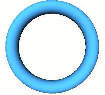
The torus is an example of a tubular boundary with MA a circle and constant r value. In Figure 1 such a circle has been approximated by 50 line segments. This produces a boundary which appears fairly smooth, and consists of 100 boundary surfaces: one cylinder for each linear segment, and one sphere patch between each adjacent pair of cylinders.

Figure 1 : MAT as an Annulus and corresponding Torus object.

Example 2 : The Ring Cyclide

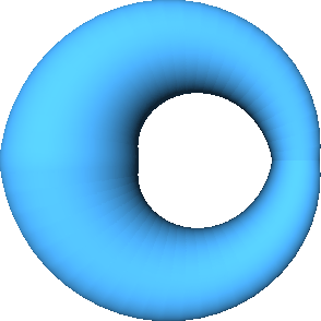
The ring cyclide is another example of a tubular boundary with a circle for its MA. Now, however, the r function increases around half the circle and then decreases again to its original value. This MAT and its boundary are shown in Figure 2. Again the circle has been approximated with 50 line segments. In this case, though, the boundary has 99 patches: one cone for each linear segment, and one sphere patch between each adjacent pair of cones except the pair at the minimal value of r. The sphere at this point is contained entirely inside the boundary.

Figure 2 : MAT as an Annulus and corresponding Cyclide object.

Example 3 : Self-intersecting Plane Curve

The alpha curve in Figure 3 shows an example of a curve with a junction of four edges. Because we have chosen to use a constant radius function along the curve, the direction vectors related to each MAT line segment are perpendicular to the line segment itself. Because of this, at the vertex where the four edges come together, the MA edges must make right angles with each other in order to keep the boundary related to a point on the MAT from crossing over the MA.

Figure 3 : Plane curve with a 4 edge junction.

Example 4 : The Helix

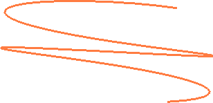
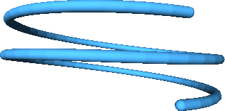
Our first example of a space curve is the helix shown in Figure 4. The helix has a constant r function associated with it, and is approximated by 80 line segments, thus it has 161 related boundary patches.

Figure 4 : Space curve - the Helix.

Example 5 : The Lemniscate of Gerono

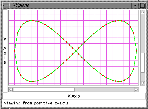
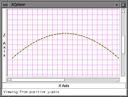
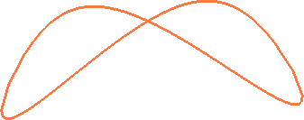
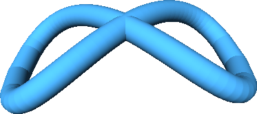
A second space curve example is shown in Figures 5 and 6. This is the Lemniscate of Gerono, with the z-coordinate given by cos x . In this example r is constant. The lemniscate is approximated by 80 line segments and has 160 related boundary patches. In Figure 5 the projections of the MAT to the xy and to the xz planes are shown. Note how the spacing of the points is not uniform in the xy plane. This is the reason for the variation in smoothness of the generated boundary tube.

Figure 5 : Lemniscate - Projections of the MAT in the XY and ZX planes.

Figure 6 : The MAT as a Leminiscate in 3Dand the corresponding object.

Back         Top         Next