A convolution is a
generic form of blending of two functions.
More precisely: a "convolution is an integral that expresses the amount of overlap of one function g as it is shifted over another function f ."
The convolution of 1D signals is typical in the filtering of sounds (local copy).
The convolution
of 2D images is the basis of image smoothing, gradient and edge
filtering (local copy).
Illustrations : www.cmap.polytechnique.fr/~peyre/adtf/illustrations/
Illustrations : www.cmap.polytechnique.fr/~peyre/adtf/illustrations/
N.B.: In a discrete world, i.e., with digital images made of
pixels, integrals are replaced (approximated) by sums.
Smoothing & noise removal
"Smoothing" is a typical form of filtering:
- the blending of one kernel (usually a "small" function) with a target function ("large" one), usually taken to be the image source.
It is used with the goal of
averaging the pixel values of the
source with a weighted sum of it surrounding neighboring pixels.
A typical form of the
smoothing kernel is to have large central values, surrounded by ever
decreasing ones. Applying convolution of the kernel to the source
therefore preserving somewhat the central pixel (source) value, by
modifying it with an averaged sum of the reduced values of its
surrounding neighbors.
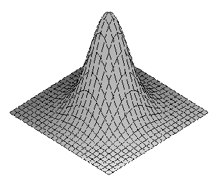
A classical example in filtering is the Gaussian kernel:
G(x) = a EXP^(-b(x-c)^2)
N.B.: it is the probability
function of the normal distribution (in statistics).

2D Gaussian kernel
Examples:
- An introduction to smoothing: http://www.mrc-cbu.cam.ac.uk/Imaging/Common/smoothing.shtml
- Correcting defects and
smoothing: http://www.reindeergraphics.com/tutorial/chap2/defect03.html
N.B.: Linearity:
It does not mean: “having the properties of a line.”
- A system is linear
if it is:
- Homogenous: If we scale the input, then the output is scaled by the same amount: f(a x) = a f(x) .
- Additive: If we add a pair of inputs
the output will be equivalent to the sum of their respective outputs:
f(x1 + x2) = f(x1) + f(x2) .
Example: Gaussian (averaging) filtering is linear (integration is linear).
Example of Non-linear filtering: the median filter.
The
median is calculated by first
sorting all the pixel values from the
surrounding neighbourhood into numerical order and then replacing the
pixel being considered with the middle pixel value.
Examples:
- 1D median filter: http://rkb.home.cern.ch/rkb/AN16pp/node168.html
- 2D median filter: http://www.dca.fee.unicamp.br/dipcourse/html-dip/c9/s3/front-page.html
Gradient filtering & Edge detection
"Gradient filtering" is a
typical way of enhancing the heterogeneous zones of a signal (1D) or
image (2D).
By gradient, it is meant
that a derivative (or differences) is sought. This is approximated by
convolving the source image with kernels which emphasize zones of rapid
change in intensity.
Furthermore, directionality is usually emphasized to bring out edges which together can trace thick lines or curves, ideally located where the eye perceives contours.
Furthermore, directionality is usually emphasized to bring out edges which together can trace thick lines or curves, ideally located where the eye perceives contours.
Examples:
- Edge detection tutorial: http://www.pages.drexel.edu/~weg22/edge.html
- (moderately) Advanced edge detection: http://www.reindeergraphics.com/tutorial/chap3/enhance04.html
Fourier Transforms & Frequency representation
A Fourier
transform is a
representation of some function in terms of a
set of sine-waves. The set of sine-waves of different frequencies is
orthogonal
(linearly independent), and it can be shown that any
continuous function can be represented by summing enough sine-waves of
the appropriate frequency, amplitude and phase (Fourier's theorem).
If I(x,y) denotes a digital
image (with pixels (x,y)), its Fourier transform (or FT) is denoted
F(u,v) where u and v typically represent the horizontal and vertical
frequency components of each sine-wave used to encode the image I.
Thus, the spatial frequency of a sine-wave can be represented (located) in a 2D u-v plane. But, we need to represent 2 more parameters for each sine-wave: its amplitude (or height) and its phase (its shift w/r to the origin).
Typically, only the magnitude is displayed; i.e., as an intensity value in the 2D vectored image indicating the sine-wave spatial frequency.
Examples:
- 1D Fourier transform: http://www.ysbl.york.ac.uk/~cowtan/fourier/ftheory.html
- 2D examples:
- FT in Crystallography, by Kevin Cowtan:
http://www.ysbl.york.ac.uk/~cowtan/fourier/gallery.html
- Intro to FT for Image Processing, by John M. Brayer: http://www.cs.unm.edu/~brayer/vision/fourier.html
- Image filtering in the
Frequency Domain:
http://local.wasp.uwa.edu.au/~pbourke/other/imagefilter/
(by Paul Bourke)
http://local.wasp.uwa.edu.au/~pbourke/other/imagefilter/
(by Paul Bourke)
References
[Milewski:Fourier]
Milewski, B., "The Fourier Transform," http://www.relisoft.com/Science/Physics/sound.html
Free software: Frequency analyzer from Relisoft: http://www.relisoft.com/freeware/
Free software: Frequency analyzer from Relisoft: http://www.relisoft.com/freeware/
[Smith:MathsDFT:2004]
Smith, J. O., "Mathematics of the
Discrete Fourier Transform (DFT) --- with Music and Audio
Applications," 2004.
http://ccrma-www.stanford.edu/~jos/r320/
http://ccrma-www.stanford.edu/~jos/r320/